Processing genetic data

\[\\[0.5in]\]

Here we process the 83 brain volume GWAS summary statistics created in a previous step. The code displayed below prepares the data for subsequent analyses, and performs data visualisation and sanity checks.

\[\\[1in]\]

---

1. Munge files as expected by Genomic SEM software

### this script will munge the gwas files using GenomicSEM

# load dependencies
library(tidyr)
library(data.table)
library(devtools)
library(GenomicSEM)
library(stringr)

# set wd to where formatted files are saved
setwd("/mnt/lustre/groups/ukbiobank/Edinburgh_Data/usr/anna/PhD/output/regenie/step2/")

hm3<-"/scratch/users/k1894405/genetic_networks/data/w_hm3.noMHC.snplist"


# list gwas files you want to munge
gwas_files<-list.files(pattern="GWAS_22chr_noTBVcontrol_")
print(length(gwas_files))

                        

for (i in gwas_files){
        # define file to be munged
            files<-i
            print(files)
        
        # name the file
            trait_name <- str_remove(i, pattern = "GWAS_22chr_noTBVcontrol_")
            trait_name <- str_remove(trait_name, pattern = ".txt")

            trait.names<-trait_name
            print(trait.names)
        
        # munge
            munge(files=files,
                    hm3=hm3,
                    trait.names=trait.names,
                    info.filter = 0.9)
}

After munging the files have 1,172,487 remaining rows (SNPs).

• 9932681 rows present in the full sumstats file

• 8737179 rows were removed as the rs-ids for these rows were not present in the reference file (HapMap3)

• 3070 rows were removed due to the effect allele (A1) column not matching A1 or A2 in the reference file

• 1599 rows were removed due to the other allele (A2) column not matching A1 or A2 in the reference file

• 8728 rows were removed due to INFO values below the designated threshold of 0.9

• 9618 rows were removed due to missing MAF information or MAFs below the designated threshold of 0.01

• 1172487 remaining rows in the sumstats

---

2. Calculate LDSC

### after formatting and munging the gwas files, I have manually transferred the files into a folder called "GWAS_munged"

library(stringr)
library(devtools)
library(GenomicSEM)

# set wd to the munged GWAS folder
setwd("/mnt/lustre/groups/ukbiobank/Edinburgh_Data/usr/anna/PhD/output/genetic_networks_project/gwas_munged/")

# specifications for ldsc function
traits<-list.files(pattern=".sumstats.gz")

# double check that 83 files have been read in 
if(length(traits) !=83){print("You are not including 83 files");break}

# no sample or population prevalence needed because brain volumes are continuous traits
# specify NA for both
desired_length<-length(traits)
sample.prev<-rep(NA, desired_length)
print(sample.prev)
population.prev<-rep(NA, desired_length)
print(population.prev)

# ld scores and weights previously downloaded (European population)
ld<-"/scratch/users/k1894405/genetic_networks/data/eur_w_ld_chr/"
wld<-"/scratch/users/k1894405/genetic_networks/data/eur_w_ld_chr/"


gwas_munged<-list.files(pattern=".sumstats.gz")
gwas_munged<-str_replace(gwas_munged,pattern=".sumstats.gz",replacement="")
trait.names<-gwas_munged

# double check that trait.names and traits match up
# first build a data set from the vectors, then compare the two vectors
test<-data.frame(trait.names,traits)
print(test)


count<-0

for(i in 1:nrow(test)){
    # which trait are we testing
        print(substr(test$traits[i], 1, nchar(as.character(test$trait.names[i]))))
        print(as.character(test$trait.names[i]))
    # break the loop if trait.names and traits don't match
        if(as.character(test$trait.names[i]) != substr(test$traits[i], 1, nchar(as.character(test$trait.names[i])))){"Trait names and trait files don't match";break}
        
        count<-count+1
        print(paste0("This is the ",count,"st/nd trait iteration"))
    }


LDSCoutput_wholebrain<-ldsc(traits=traits,
                             ld=ld,wld=wld,
                             trait.names = trait.names,
                             ldsc.log="/mnt/lustre/groups/ukbiobank/Edinburgh_Data/usr/anna/PhD/output/genetic_networks_project/ldsc/ldsc_wholebrain.log",
                             sample.prev=sample.prev,
                             population.prev=population.prev,
                             stand=T)

## save output for subsequent analyses
save(LDSCoutput_wholebrain, file="/mnt/lustre/groups/ukbiobank/Edinburgh_Data/usr/anna/PhD/output/genetic_networks_project/ldsc/ldsc_wholebrain.RData")

---

3. Plot heatmaps

## this script is displaying the heatmaps of the networks
rm(list=ls())
# load dependencies
library(stringr)
library(reshape2)
library(ggplot2)

# load data and name it according to network
workingwd<-getwd()
temporarywd<-paste0(workingwd,"/data_my_own/ldsc/")
setwd(temporarywd)

networks<-list.files(pattern=".RData")
network_names<-str_replace(networks,pattern=".RData",replacement = "")

for(i in 1:length(networks)){
load(networks[i])
  name<-network_names[i]
  assign(name,LDSCoutput)
}

## name all columns in S_Stand after brain regions and round S_Stand
for(i in network_names){
  output<-get(i)
  dimnames(output$S_Stand)[[1]]<-dimnames(output$S)[[2]]
  dimnames(output$S_Stand)[[2]]<-dimnames(output$S)[[2]]
  name<-i
  assign(name,output)
  output$S_Stand<-round(output$S_Stand,digits = 2)
  name_cor<-paste0("cor_",i)
  assign(name_cor,output$S_Stand)
}

# count number of correlation matrices
#length(ls(pattern="cor_"))

# create vector containing names of the correlation matrices
matrices<-ls(pattern="cor_")

## plot the rounded correlation matrices


# get lower triangle of matrix

get_lower_tri<-function(cormatrix){
    cormatrix[upper.tri(cormatrix)] <- NA
    return(cormatrix)
} 

for(i in matrices){
  cormatrix<- get(i)
  
  lower_triangle<-get_lower_tri(cormatrix)
  lower_triangle<-reshape2::melt(lower_triangle)
  #print(i)
  #print(lower_triangle)
  lower_triangle$value<-ifelse(lower_triangle$value >1,1,lower_triangle$value)
  
  heatmap<-
    ggplot(data=lower_triangle, aes(Var1,Var2,fill=value))+
    geom_tile(color = "white")+
    theme_minimal()+ 
    theme_bw()+
    theme(axis.text.x = element_text(angle = 45, vjust = 1, 
                                     size = 8, hjust = 1))+
    theme(axis.text.y = element_text(vjust = 1, 
                                     size = 8, hjust = 1))+
    theme(axis.title.x=element_blank(),
          axis.title.y = element_blank(),
          panel.grid.major = element_blank(),
          panel.border = element_blank(),
          axis.ticks = element_blank(),
          legend.justification = c(1,0),
          #legend.position = c(0.45,0.7),
          legend.direction = "horizontal")+  
    scale_fill_gradient2(low="royalblue1",high="palevioletred",mid ="white",
                         midpoint=0,limit=c(-1,1),na.value="white",
                         name="Genetic\ncorrelation")+
    guides(fill=guide_colorbar(barwidth = 7,barheight = 1,title.position = "top",title.hjust = 0.5))+
    coord_fixed()
  
  heatmap<-heatmap+
    geom_text(aes(Var1,Var2,label=value),color="black",size=2)
  
  name<-paste0(i,"_heatmap")
  assign(name,heatmap)
}

Example correlation matrices for three networks inferred through LDSC

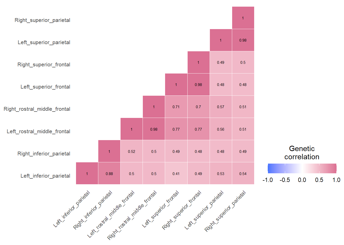
Central Executive

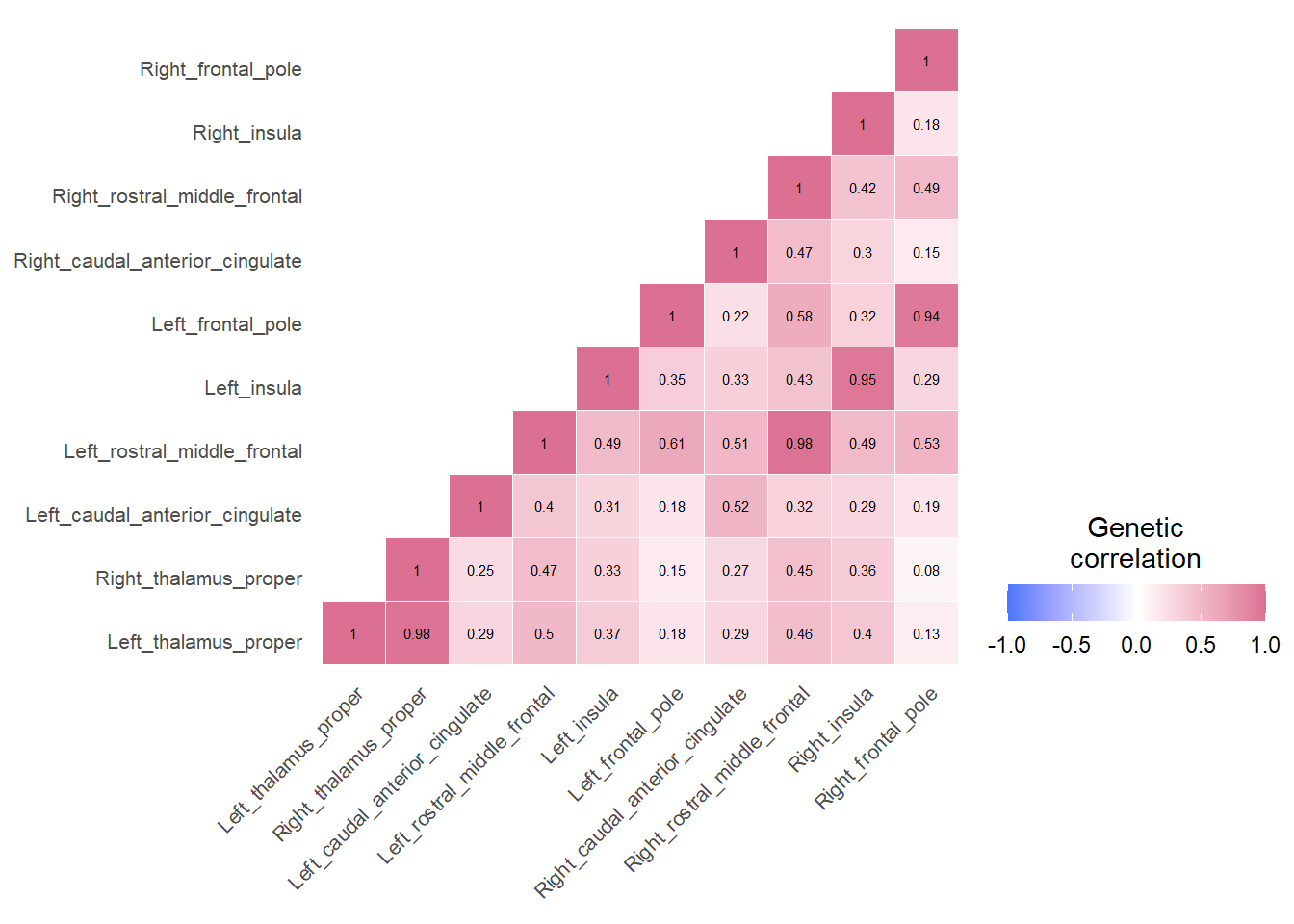
Cingulo-opercular

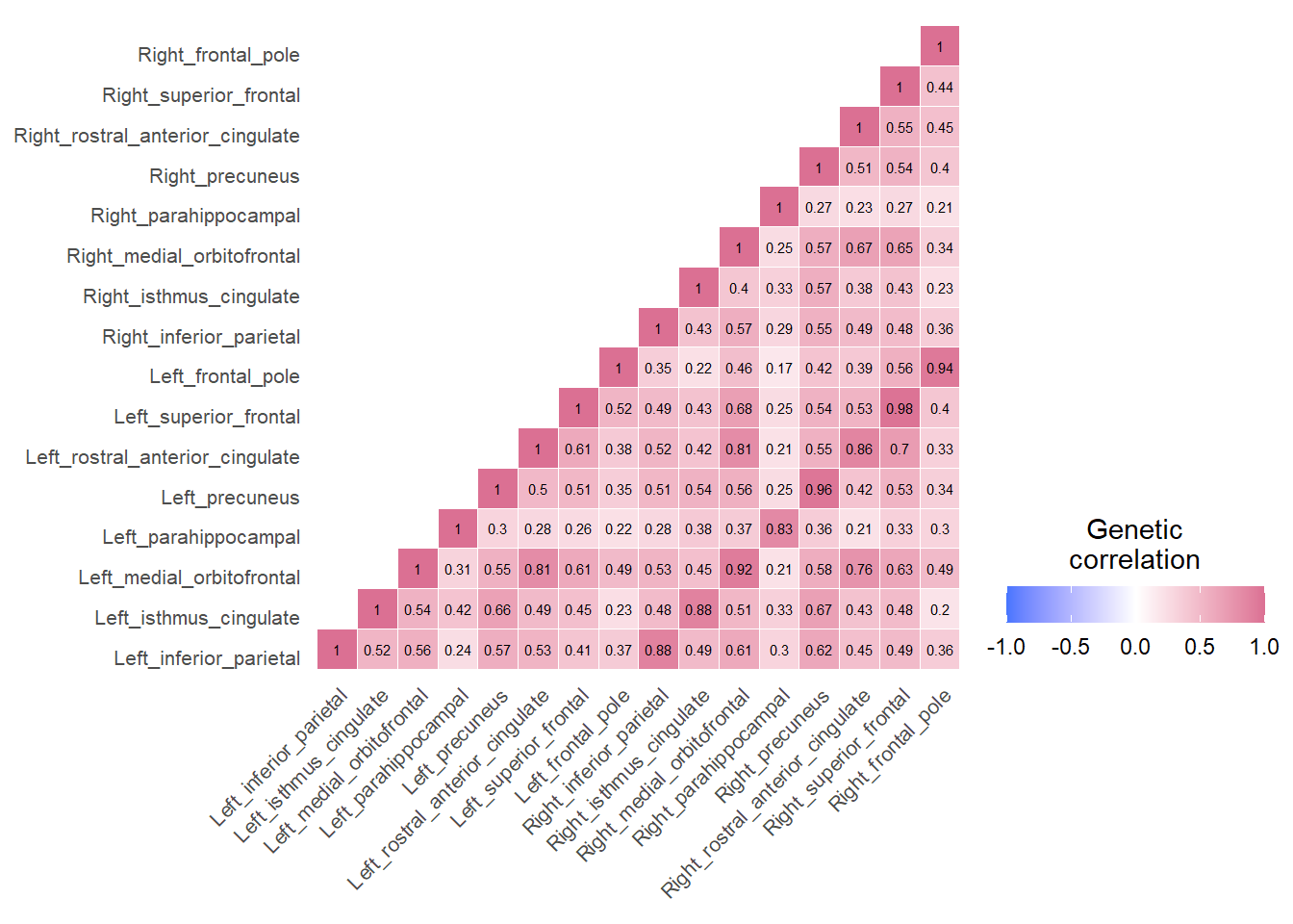
Default Mode

Plot heatmap for genetic correlations across the whole brain

# set working directory
workingd<-getwd()
temporarywd<-paste0(workingd,"/data_my_own/ldsc/")
setwd(temporarywd)


load("whole_brain.RData")
ldscoutput<-LDSCoutput_wholebrain
dimnames(ldscoutput$S_Stand)[[1]]<-dimnames(ldscoutput$S)[[2]]
dimnames(ldscoutput$S_Stand)[[2]]<-dimnames(ldscoutput$S)[[2]]
whole_brain_corr<-reshape2::melt(ldscoutput$S_Stand)
whole_brain_corr$value_corrected<-ifelse(whole_brain_corr$value>1,1,whole_brain_corr$value)

  heatmap<-
    ggplot(data=whole_brain_corr, aes(Var1,Var2,fill=value_corrected))+
    geom_tile(color = "white")+
    theme_minimal()+ 
    theme_bw()+
    theme(axis.text.x = element_blank())+
    theme(axis.text.y = element_blank())+
    theme(axis.title.x=element_blank(),
          axis.title.y = element_blank(),
          panel.grid.major = element_blank(),
          panel.border = element_blank(),
          axis.ticks = element_blank(),
          legend.justification = c(1,0),
          #legend.position = c(0.45,0.7),
          legend.direction = "horizontal")+  
    scale_fill_gradient2(low="royalblue1",high="palevioletred2",mid ="white",
                         midpoint=0,limit=c(-1,1),na.value="white",
                         name="Genetic\ncorrelation")+
    guides(fill=guide_colorbar(barwidth = 7,barheight = 1,title.position = "top",title.hjust = 0.5))+
    coord_fixed()
  heatmap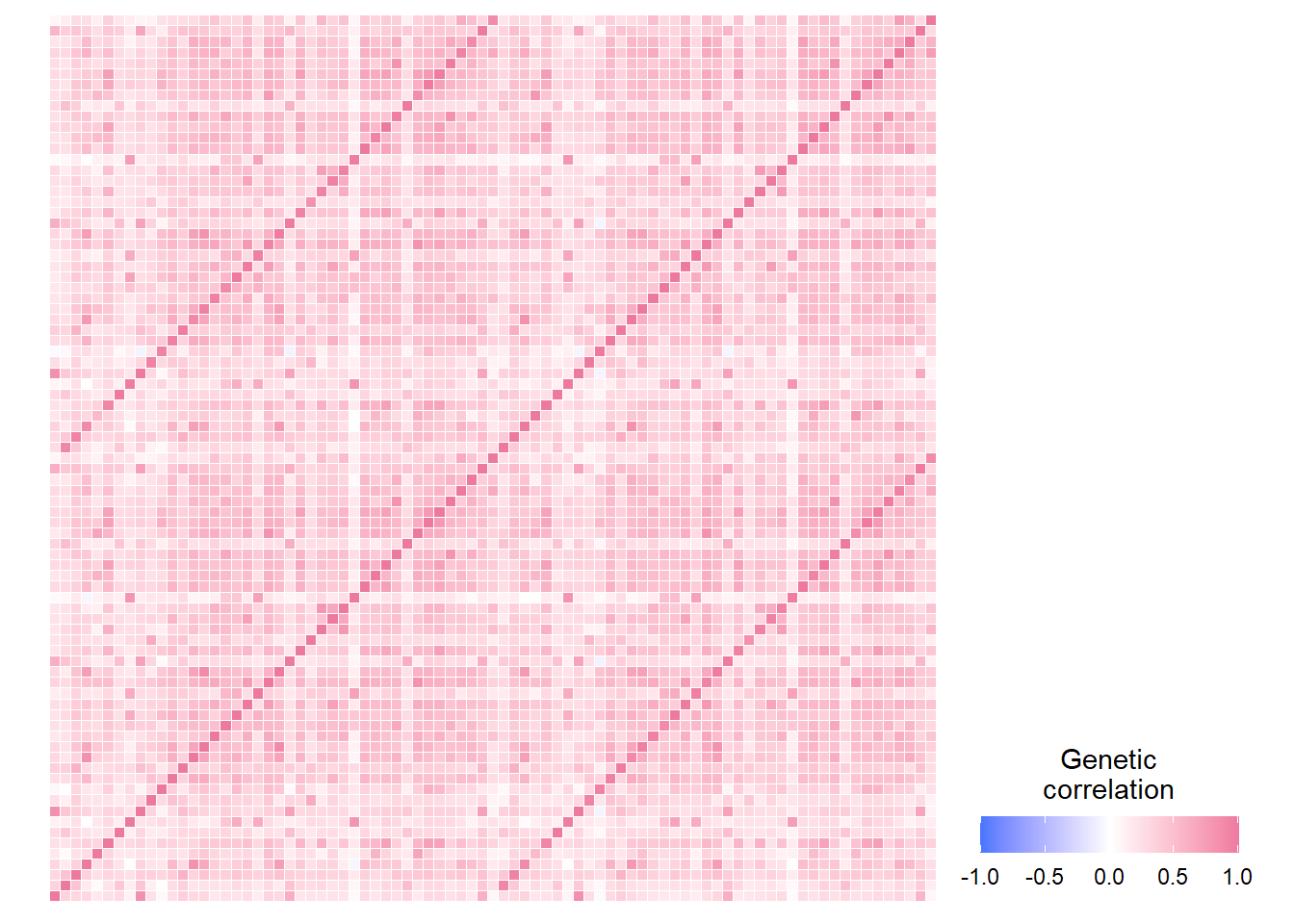

The vertical line through the diagnonal indicates the genetic correlation of a brain area with itself, and the vertical lines that run parallel to it indicate the strong genetic correlation with their contralateral counterpart. The only region that does not exhibit this bilateral symmetry is the brain stem.

Code for heatmaps in Supplementary Materials

### whole brain
tiff("heatmap_whole_brain.tiff", width = 7, height = 6, units = 'in', res=1000)
heatmap
dev.off()


### central executive
tiff("heatmap_central_exec.tiff", width = 6, height = 6, units = 'in', res=1000)
cor_central_exec_heatmap
dev.off()

### cingulo
tiff("heatmap_cingulo.tiff", width = 6, height = 6, units = 'in', res=1000)
cor_cingulo_heatmap
dev.off()

### default mode
tiff("heatmap_default.tiff", width = 7, height = 7, units = 'in', res=1000)
cor_default_mode_heatmap
dev.off()

### hippocampal
tiff("heatmap_hippocampal.tiff", width = 6, height = 6, units = 'in', res=1000)
cor_hippocampal_heatmap
dev.off()

### Multiple demand
tiff("heatmap_multiple.tiff", width = 6, height = 6, units = 'in', res=1000)
cor_multiple_heatmap
dev.off()


### P-FIT
tiff("heatmap_p_fit.tiff", width = 10, height = 10, units = 'in', res=1000)
cor_p_fit_heatmap
dev.off()

### Salience
tiff("heatmap_salience.tiff", width = 6, height = 6, units = 'in', res=1000)
cor_salience_heatmap
dev.off()

### Sensorimotor
tiff("heatmap_sensorimotor.tiff", width = 6, height = 6, units = 'in', res=1000)
cor_sensori_heatmap
dev.off()

### temporo
tiff("heatmap_temporo.tiff", width = 10, height = 10, units = 'in', res=1000)
cor_temporo_heatmap
dev.off()

---

Sanity checks

Plot standard errors

Here we display the standard errors for the lower triangle of the genetic correlation matrix.

temporarywd<-paste0(workingd,"/data_my_own/ldsc/")
setwd(temporarywd)

load("whole_brain.RData")
ldscoutput<-LDSCoutput_wholebrain


k<-nrow(ldscoutput$S)
SE<-matrix(0, k, k)
SE[lower.tri(SE,diag=TRUE)] <-sqrt(diag(ldscoutput$V))

  dimnames(SE)[[1]]<-dimnames(ldscoutput$S)[[2]]
  dimnames(SE)[[2]]<-dimnames(ldscoutput$S)[[2]]

get_lower_tri<-function(cormatrix){
  cormatrix[upper.tri(cormatrix)] <- NA
  return(cormatrix)
}

SE_lower<-get_lower_tri(SE)
SE_lower<-reshape2::melt(SE_lower)


###############################################
##### plot all SEs across the entire brain

library(ggridges)

ggplot(SE_lower, aes(value,color="indianred2",fill="indianred2"))+
  geom_density(show.legend=FALSE)+
              theme_ridges()+
              scale_x_continuous(n.breaks = 5)+
              xlab("Standard errors of genetic correlations")+ylab("")+
              theme(legend.position = "none",
                    axis.text.x = element_text(size=24),
                    axis.text.y = element_text(size=24),
                    axis.title.x = element_text(size=26),
                    panel.background = element_blank(), 
                    axis.line = element_line(color="black"), 
                    axis.line.x = element_line(color="black"))+theme_bw()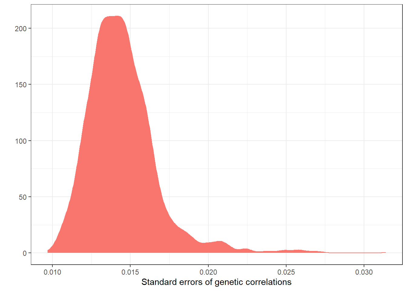

Standard errors of the genetic correlation estimates have an average of 0.014 (SD = 0.002), and range between 0.01 and 0.031.

Display genetic correlations

library(plyr)
library(TeachingDemos)
source("https://raw.githubusercontent.com/talgalili/R-code-snippets/master/boxplot.with.outlier.label.r")

# load whole brain data
workingd<-getwd()
temporarywd<-paste0(workingd,"/data_my_own/ldsc/")
setwd(temporarywd)

load("whole_brain.RData")
ldscoutput<-LDSCoutput_wholebrain
  dimnames(ldscoutput$S_Stand)[[1]]<-dimnames(ldscoutput$S)[[2]]
  dimnames(ldscoutput$S_Stand)[[2]]<-dimnames(ldscoutput$S)[[2]]

  lower_triangle<-get_lower_tri(ldscoutput$S_Stand)
  diag(lower_triangle)<-NA
  lower_triangle<-reshape2::melt(lower_triangle)
  
lower_triangle$jointname<-paste(lower_triangle$Var1,lower_triangle$Var2)


boxplot.with.outlier.label(lower_triangle$value,NA,xaxt="n",yaxt="n",ylab="LDSC coefficient",ylim=c(-0.8,1.2),main="Variation in LDSC coefficients\namong 83 traits",spread_text = F)
axis(side=2,las=2)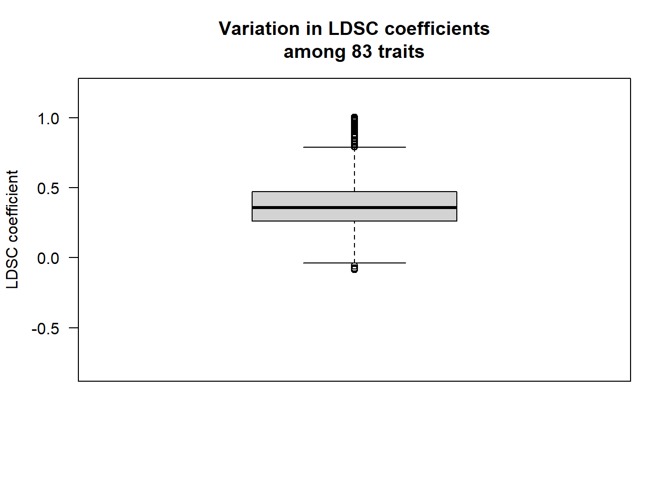

# display the lower correlations
#lower_triangle$jointname<-ifelse(lower_triangle$value<=-0.25,lower_triangle$jointname,NA)

display<-lower_triangle[which(!is.na(lower_triangle$value)),c("Var1","Var2","value")]
display$value<-round(display$value, digits=2)
names(display)<-c("Volume 1","Volume 2","Genetic correlation")


library(knitr)
#kable()
library(DT)
datatable(display, rownames=FALSE, filter="top",options= list(pageLength=5,scrollX=T))

# work out which correlations are above 1 and below 0
traits_corr_above1<-as.data.frame(lower_triangle[which(lower_triangle$value >1.0000000001),c("Var1","Var2","value")])
traits_corr_below0<-lower_triangle[which(lower_triangle$value<0),c("Var1","Var2","value")]

Note that we found correlations slightly above 1 for the following traits:
Right_DC & Left_DC; Right_precentral & Left_precentral.

Negative genetic correlations

# work out CIs for negative correlations
SE_lower_comp<-SE_lower
names(SE_lower_comp)<-c("Var2","Var1","SE")
df<-merge(traits_corr_below0,SE_lower_comp,by=c("Var1","Var2"),all=T)


## after merging the correlations below 1 and the SEs, some genetic correlations have not been assigned an SE because the brain volumes have been flipped (Var1 vs. Var2)
# In the following loop we identify these traits, flip them, and assign the standard error to the entry with the non-missing genetic correlation 
for(i in df$Var1[which(is.na(df$SE) & !is.na(df$value))]){
  for(j in df$Var2[which(is.na(df$SE) & !is.na(df$value))]){
    df[which(df$Var1 == i & df$Var2 ==j),"SE"]<-df[which(df$Var1 == j & df$Var2 ==i),"SE"]
  }
}

neg_cor_with_SE<-df[which(!is.na(df$value)),]
# calculate CIs 95%
neg_cor_with_SE$CI95<-paste(round(neg_cor_with_SE$value-(1.96*neg_cor_with_SE$SE),digits = 3)," - ", round(neg_cor_with_SE$value+(1.96*neg_cor_with_SE$SE),digits=3))

kable(neg_cor_with_SE[,c("Var1","Var2","value","CI95")], digits = 3, row.names = F, col.names = c("Volume 1","Volume 2","Genetic correlation","95% CI"), caption = "Negative Genetic Correlations")

Negative Genetic Correlations

Volume 1	Volume 2	Genetic correlation	95% CI
Left_cuneus	Left_bankssts	-0.008	-0.035 - 0.019
Left_pericalcarine	Left_bankssts	-0.060	-0.087 - -0.032
Right_bankssts	Left_pericalcarine	-0.008	-0.035 - 0.019
Right_caudal_anterior_cingulate	Left_pericalcarine	-0.009	-0.031 - 0.014
Right_cuneus	Left_bankssts	-0.010	-0.036 - 0.017
Right_frontal_pole	Brain_stem	-0.037	-0.062 - -0.012
Right_frontal_pole	Left_DC	-0.075	-0.099 - -0.051
Right_frontal_pole	Left_pallidum	-0.083	-0.11 - -0.057
Right_frontal_pole	Right_DC	-0.073	-0.098 - -0.048
Right_pallidum	Right_frontal_pole	-0.072	-0.097 - -0.046
Right_pericalcarine	Left_bankssts	-0.008	-0.036 - 0.02

# negative genetic correlations
neg_cor<-sum(neg_cor_with_SE$value<=0 & !is.na(neg_cor_with_SE$value))
total_cor<-(83*(83-1))/2
percent_neg<-round((neg_cor/total_cor)*100,digits = 2)

Genetic correlations are negative in 0.32% of the cases (negative correlations = 11, total correlations = 3403).

As you can see in the table below, nearly all negative correlations involve either the frontal pole or the bankssts, which are both known to be difficult to segment, and therefore could potentially index noise (which could explain the negative correlations with more reliably measured brain volumes).

---

Data display in manuscript

Boxplots displaying SNP-heritabilites and genetic correlations

library(readr)
library(tidyr)
library(ggplot2)
library(Hmisc)
library(plyr)
library(RColorBrewer)
library(reshape2)
library(PupillometryR)
library(cowplot)
# plotted with explanation on : https://micahallen.org/2018/03/15/introducing-raincloud-plots/


#tiff("boxplots.tiff", width = 9, height = 6, units = 'in', res=1000)

##########################################
## Plot SNP-heriability
#########################################
# data to be plotted: heritability estimates
workingd<-getwd()
temporarywd<-paste0(workingd,"/data_my_own/ldsc/")
setwd(temporarywd)

heritability<-read.table("heritability_brain_volumes_14052021.txt",header=T)

heritability$name<-rep("SNP-heritability",83)
heritability$outlier<-NA

# plot SNP-heritability
plot_heritability<-
                  ggplot(data=heritability,aes(x=name,y=h2_obs))+
                  geom_flat_violin(position = position_nudge(x = .2, y = 0), alpha = .8, fill="gray85",alpha=0.1) +
  geom_point(aes(y = h2_obs), position = position_jitter(width = .15), size = .5, alpha = 1,colour="gray65")+
  geom_boxplot(width = .2, guides = FALSE, outlier.shape = NA, alpha = 0.5)+ 
  geom_text(aes(label = outlier), na.rm = TRUE, hjust = 1.1, vjust=-1.2, colour="gray65",size=3.5)+
   expand_limits(x=2)+
  theme_bw() +
  theme(text = element_text(size=12),
        axis.text.x = element_blank(),
        axis.text.y = element_text(size=13),
        axis.title.y = element_text(face="bold", colour='black', size=17),
        axis.title.x = element_blank())+
  ylab("SNP-heritability")

##################################################
# Plot genetic correlations
#################################################
temporarywd<-paste0(workingd,"/data_my_own/ldsc/")
setwd(temporarywd)

load("whole_brain.RData")
ldscoutput<-LDSCoutput_wholebrain
  dimnames(ldscoutput$S_Stand)[[1]]<-dimnames(ldscoutput$S)[[2]]
  dimnames(ldscoutput$S_Stand)[[2]]<-dimnames(ldscoutput$S)[[2]]

  get_lower_tri<-function(cormatrix){
  cormatrix[upper.tri(cormatrix)] <- NA
  return(cormatrix)
  }
  
  lower_triangle<-get_lower_tri(ldscoutput$S_Stand)
  # remove correlations with oneself
  diag(lower_triangle)<-NA
  #melt correlation matrix
  lower_triangle<-reshape2::melt(lower_triangle)
  # remove correlations with itself
  lower_triangle$value<-ifelse(lower_triangle$Var1 == lower_triangle$Var2,NA,lower_triangle$value)

lower_triangle$jointname<-paste(lower_triangle$Var1,lower_triangle$Var2)
lower_triangle$name<-rep("genetic corr",nrow(lower_triangle))


# we only keep lower_triangle values that are not missing
lower_triangle<-lower_triangle[which(!is.na(lower_triangle$value)),]

## plot genetic correlations
plot_genetic_corr<-
                  ggplot(data=lower_triangle,aes(x=name,y=value))+
                  geom_flat_violin(position = position_nudge(x = .2, y = 0), alpha = .8,fill="gray85",alpha=0.6) +
                  geom_point(aes(y = value), position = position_jitter(width = .15), size = .5, alpha = 0.9,colour="gray65") +
                  geom_boxplot(width = .2, guides = FALSE, outlier.shape = NA, alpha = 0.5)+
                  expand_limits(x=2)+
                  theme_bw()+
                  theme(text = element_text(size=12),
                        axis.text.x = element_blank(),
                        axis.text.y = element_text(size=13),
                        axis.title.y = element_text(face="bold", colour='black', size=17),
                        axis.title.x = element_blank())+
                  ylab("Genetic correlations")+
                  ylim(-0.4,1)

#############################################################################################
# make same plot for phenotypic correlations
# code for how we obtain the cor_matrix on the Edinburgh server can be found in this document under "Pre-processing: Phenotypic data"
temporarywd_pheno<-paste0(workingd,"/data_my_own/Pheno_preparation/")
setwd(temporarywd_pheno)

load("pheno_decomposition.RData")

lower_triangle_pheno<-get_lower_tri(cor_matrix)
# remove correlations with oneself
diag(lower_triangle_pheno)<-NA
#melt
lower_triangle_pheno<-reshape2::melt(lower_triangle_pheno)
lower_triangle_pheno$value<-ifelse(lower_triangle_pheno$Var1 == lower_triangle_pheno$Var2,NA,lower_triangle_pheno$value)

# we only keep non-missing values
lower_triangle_pheno<-lower_triangle_pheno[which(!is.na(lower_triangle_pheno$value)),]

# add variable to plot against
lower_triangle_pheno$name<-rep("phenotypic corr",nrow(lower_triangle_pheno))

## plot phenotypic correlations
plot_phenotypic_corr<-
                  ggplot(data=lower_triangle_pheno,aes(x=name,y=value))+
                  geom_flat_violin(position = position_nudge(x = .2, y = 0), alpha = .8,fill="gray85",alpha=0.6) +
                  geom_point(aes(y = value), position = position_jitter(width = .15), size = .5, alpha = 0.9,colour="gray65") +
                  geom_boxplot(width = .2, guides = FALSE, outlier.shape = NA, alpha = 0.5)+
                  expand_limits(x=2)+
                  theme_bw()+
                  theme(text = element_text(size=12),
                        axis.text.x = element_blank(),
                        axis.text.y = element_text(size=13),
                        axis.title.y = element_text(face="bold", colour='black', size=17),
                        axis.title.x = element_blank())+
                  ylab("Phenotypic correlations")+
                  ylim(-0.4,1)
#############################################################################################
# display all three plots together
plot_grid(plot_heritability,plot_genetic_corr,plot_phenotypic_corr,ncol=3,nrow=1,labels = c("A","B","C"))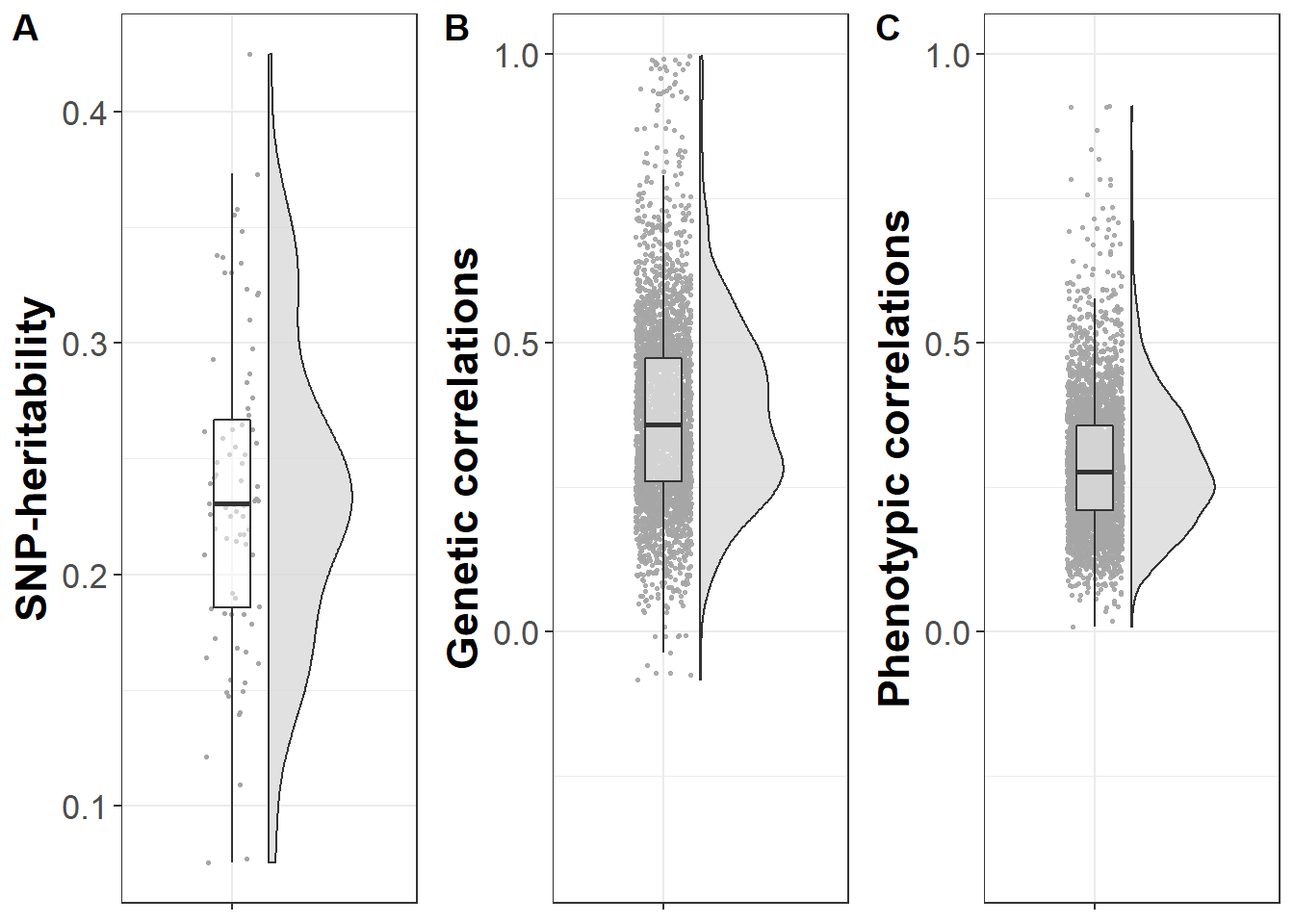

#setwd(workingd)
#dev.off()

 

---

By Anna Elisabeth Fürtjes

anna.furtjes@kcl.ac.uk