GWAS calculation
Here, we calculate the genome-wide association study summary statistics for each of our 83 brain volumes. The input data used was generated with the code displayed here:
We used the regenie software for the calculation.
\[\\[0.5in]\]
Regenie Step 1
#!/bin/bash -l

#SBATCH --mem=16G
#SBATCH --nodes=1
#SBATCH --ntasks=16
#SBATCH --partition brc,shared
#SBATCH --output=~/anna/PhD/output/regenie/step2regenie.out
#SBATCH --job-name=regenie


# set input paths
cleandatapathpheno=~/anna/PhD/output/pheno_preparation/
cleandatapathgeno=~/anna/PhD/output/geno_qc/
ukbpath=/scratch/datasets/ukbiobank/ukb18177/


# set output paths
outputpath=~/anna/PhD/output/regenie/
scriptspath=~/anna/PhD/scripts/regenie/

cd  ${outputpath}

# regenie doesn't like bim files with chrom nums greater than 24
# also I don't need the X chromosome

module load apps/plink/1.9.0b6.10

plink \
--bed ${ukbpath}genotyped/ukb_binary_v2.bed  \
--bim ${ukbpath}genotyped/ukb_binary_v2.bim \
--fam ${ukbpath}genotyped/wukb18177_cal_chr1_v2_s488264.fam \
--chr 1-22 \
--make-bed \
--out ${outputpath}tmp_ukb18177_glanville_binary_pre_qc_no26X

# load regenie module
module load utilities/use.dev
module load apps/regenie/2.0.1-mkl

regenie \
  --step 1 \
  --bed ${outputpath}tmp_ukb18177_glanville_binary_pre_qc_no26X \
  --extract ${cleandatapathgeno}geneticQC_UKB_15042021__MAF0.01_GENO0.02_MIND0.02_CAUC1_UKBQC1_UNREL0.044_HWE0.00000001_SEX1.snplist \
  --phenoFile ${cleandatapathpheno}target_phenotypes_83volumes_gwas.txt \
  --keep ${cleandatapathgeno}geneticQC_UKB_15042021__MAF0.01_GENO0.02_MIND0.02_CAUC1_UKBQC1_UNREL0.044_HWE0.00000001_SEX1.fam \
  --catCovarList sex,batch \
  --maxCatLevels 106 \
  --covarFile ${cleandatapathpheno}covariates_volume_gwas.txt \
  --bsize 1000 \
  --lowmem \
  --lowmem-prefix ${outputpath}tmp_rg \
  --out ${outputpath}fit_out


### This script is an adapted version of Ryan Arathimos' script at https://github.com/applyfun/gwas_methods/blob/main/regenie_gwas_step1.sh

### sbatch -p shared,brc ~/anna/PhD/scripts/regenie/regenie_gwas_step1.sh
Note that the plink step prior to step 1 in regenie resulted in another 16,000 SNPs to be removed. Therefore, the final GWAS analysis included 571,257 out of 587,583 directly genotyped SNPs.
Regenie Step 2
#!/bin/sh -l

#SBATCH --job-name=regenie_step2
#SBATCH --partition brc,shared
#SBATCH --output=~/anna/PhD/output/regenie/step2/array_regenie.%A_%a.out
#SBATCH --cpus-per-task=8
#SBATCH --mem-per-cpu=8G
#SBATCH --array=1-22%22


cd ~/anna/PhD/scripts/regenie/

# set input paths
cleandatapathpheno=~/anna/PhD/output/pheno_preparation/
cleandatapathgeno=~/anna/PhD/output/geno_qc/
imputeddata=/mnt/lustre/groups/ukbiobank/ukb18177_glanville/imputed/

# set output paths
outputpath=~/anna/PhD/output/regenie/
scriptspath=~/anna/PhD/scripts/regenie/

# load regenie module and assign array task ID as Chromosome number
echo ${SLURM_ARRAY_TASK_ID}
CHR=${SLURM_ARRAY_TASK_ID}
echo ${CHR}

module load utilities/use.dev
module load apps/regenie/2.0.1-mkl

regenie \
  --step 2 \
  --bgen ${imputeddata}ukb18177_glanville_imp_chr${CHR}_MAF1_INFO4_v1.bgen \
  --sample ${imputeddata}ukb18177_glanville_chr1.sample \
  --covarFile ${cleandatapathpheno}covariates_volume_gwas.txt \
  --catCovarList sex,batch \
  --maxCatLevels 106 \
  --phenoFile ${cleandatapathpheno}target_phenotypes_83volumes_gwas.txt \
  --keep ${cleandatapathgeno}geneticQC_UKB_15042021__MAF0.01_GENO0.02_MIND0.02_CAUC1_UKBQC1_UNREL0.044_HWE0.00000001_SEX1.fam \
  --bsize 400 \
  --minINFO 0.4 \
  --minMAC 5 \
  --pred ${outputpath}fit_out_pred.list \
  --split \
  --out ${outputpath}step2/regenie_chr_${CHR}_out

echo Done

### This script is an adapted version of Ryan Arathimos' script at https://github.com/applyfun/gwas_methods/blob/main/regenie_gwas_step2.sh

### sbatch -p brc,shared ~/anna/PhD/scripts/regenie/regenie_gwas_step2.sh
Merge regenie output
The regenie software outputs the results for each autosomes separately. The following script merges and formats the 22 autosomes to one file and re-names some of the columns according to naming conventions.
#### merge all regenie output files

library(data.table)
library(stringr)

setwd("~/PhD/output/regenie/step2/")

ref<-fread("~/PhD/scripts/pheno_preparation/region_codes.txt",data.table=F)

# test whether all 83 traits have 22 chromosome files assigned to them
for(i in 1:nrow(ref)){
    num<-length(list.files(pattern=paste0(ref$Region[i],".regenie")))
    print(num)
    if(num != 22) {break}

    # save files names for each trait
    file_names<-list.files(pattern=paste0(ref$Region[i],".regenie"))
    vector_name<-paste0(ref$Region[i],"_files")
    print(vector_name)
    assign(vector_name, file_names)
}

# throw an error if we don't end up with 83 files
if(length(ls(pattern="_files")) != 83){"You don't have 83 files"; break}


#######################################################################
# Read in the files for each area and merge them

all_traits<-ls(pattern="_files")

for(i in all_traits){

trait_files<-get(i)

    # set object to count number of rows to 0
    expected_rows<-0

    # read in all files that belong to an area (eg. Brain stem) and save them in dat

    num<-length(trait_files)
    dat<-vector("list",num)

            print(paste0("Number of chromosomes read in for ",i))
        for(j in 1:length(trait_files)){

            print(j)
            file<-trait_files[j]
            dat[[j]]<-fread(file,header=T,data.table=F)

            # calculate number of rows we are expecting in output file
            expected_rows<-expected_rows+nrow(dat[[j]])
            }


    # merge the files by all existing columns
    merged_file<-Reduce(function(x,y) merge(x = x, y = y, by = c("CHROM","GENPOS","ID","ALLELE0","ALLELE1","A1FREQ","INFO","N","TEST","BETA","SE","CHISQ","LOG10P"), all=T), dat)

    print("Done merging chromosome files")

    ## Sanity checks: Does the resulting file have the expected dimensions?
    if(nrow(merged_file)!= expected_rows){print("Resulting merged file does not match the expected numeber of rows");break}

    if(ncol(merged_file) != 13){print("Resulting merged files does not match the expected number of columns"); break}

    print("File has dimensions as expected")
    print(dim(merged_file))

    # transform pvalues from log transformation to regular
    # https://www.biostars.org/p/358046/
    merged_file$P<-10^(-merged_file$LOG10P)
    if(min(merged_file$P,na.rm=T)<=0 | max(merged_file$P,na.rm=T) >= 1){"Transformed p-value is out of bounds"; break}

    print("Done transform p-value column, and p-values are between 0 and 1")

    # rename some of the columns (more intuitive)

    names(merged_file)[which(names(merged_file) == "ALLELE0")]<-"OA"
    names(merged_file)[which(names(merged_file) == "ALLELE1")]<-"EA"
    names(merged_file)[which(names(merged_file) == "A1FREQ")]<-"EAFREQ"

    print("Done renaming columns")

    # create MAF column
    merged_file$MAF<-ifelse(merged_file$EAFREQ < 0.5, merged_file$EAFREQ, 1-merged_file$EAFREQ))

    print(paste0("This is the file head for ",i))
    print(head(merged_file))


    # define file name to save the merged file
    region_name<-str_remove(i,pattern="_files")
    filename_print <- paste0("~/PhD/output/regenie/step2/GWAS_22chr_noTBVcontrol_", region_name)

                    # for testing
                    #   assign(region_name,merged_file)


    # save merged file
    write.table(merged_file, paste0(filename_print,".txt"), sep = "\t", row.names = FALSE, col.names = TRUE)

    print(paste0("Done writing file for ", region_name))
}


print("Done all traits")
Manhattan and quantile-quantile plot
For sanity checks of the 83 brain volume gwas, refer to the next step of this project. The qqman package was used (and slightly modified, see below) to generate these plots.
### Note:
# I have modified the manhattan function in order to print larger labels for the axes and SNP IDs
# This was not possible just by adding aestetic arguments because "cex = 1" is referred to many times in the function and R doesn't know which incidence to allocate it to
# Therefore, I needed to go in manually and change the cex arguments in the function
# To do that, I copied the manhattan source code from here: https://github.com/stephenturner/qqman/blob/master/R/manhattan.R
# into a separate document called: manhattan_big.R
# modify the cex arguments
# copy and paste the function into the console
# make sure you load the dependency "calibrate" for the textxy function
# run the code below to create pngs for each brain volume


#### citation for qqman: Turner, S.D. qqman: an R package for visualizing GWAS results using Q-Q and manhattan plots. biorXiv DOI: 10.1101/005165 (2014).

# load dependencies
library(data.table)
library(qqman)
library(stringr)
library(calibrate)

# set wd to where the gwas files are stored
setwd("/mnt/lustre/groups/ukbiobank/Edinburgh_Data/usr/anna/PhD/output/regenie/step2/")

# list all files of interest
files_of_interest <- list.files(pattern="GWAS_22chr_noTBVcontrol_")


###testing
### file<-fread("GWAS_22chr_noTBVcontrol_Left_accumbens_area.txt", header=T,data.table=F)

for(i in files_of_interest){
    # read in GWAS file
    file<-fread(i, header=T,data.table=F)
    #file<-file[c(1:1270000),]

    trait_name <- str_remove(i, pattern = "GWAS_22chr_noTBVcontrol_")
    trait_name <- str_remove(trait_name, pattern = ".txt")

    png(filename = paste0("/mnt/lustre/groups/ukbiobank/Edinburgh_Data/usr/anna/PhD/output/",trait_name,".png"), width = 1575, height=700, units="px")
    layout_matrix <- matrix(1:2, nrow = 1, ncol=2)
    layout(layout_matrix,  widths = 2:1) #heights = 1.5:1,
    par(mar=c(5, 4, 4, 2))
    par(oma = c(3,3,3,3))

    # Make MANHATTAN PLOT
    #manhattan(file, chr="CHR",bp="POS",snp="MarkerName",p="P")
    # optional: annotate SNPs with a minimum pvalue, here 0.01 is above the bottom cut-off line

    trait_name <- str_replace_all(trait_name, pattern = "_", replacement = " ")


    main = paste0("Manhattan plot: ", trait_name)
    manhattan_big(file, main = main, col = c("#e70000","#1E90FF"), chr="CHROM",bp="GENPOS",snp="ID",p="P", annotatePval=0.01, cex.axis = 1.5)

    ### Assess systematic bias in GWAS using Genomic Inflation Factor
    chisq <- qchisq(1-file$P,1)
    lambda <- median(chisq)/qchisq(0.5,1)

    # MAKE QQ PLOT
    main <- paste0("QQ plot: ", trait_name, " (Lambda = ",round(lambda,digits=3),")")
    qq(file$P, main = main, cex=1,cex.axis = 1.5)

    dev.off()
}

#dev.off()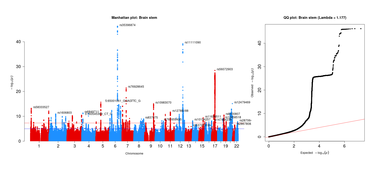
Brain stem GWAS
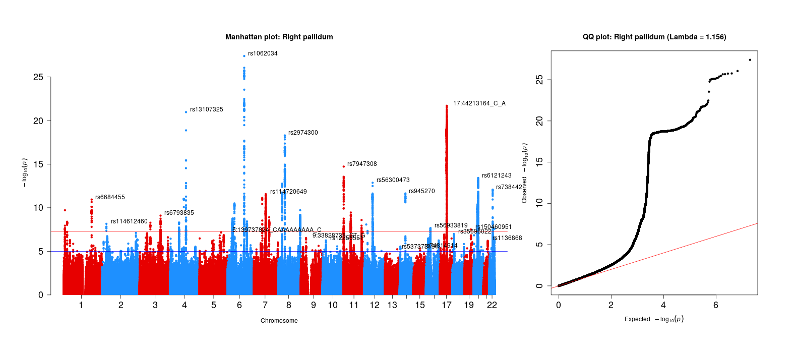
Right pallidum GWAS
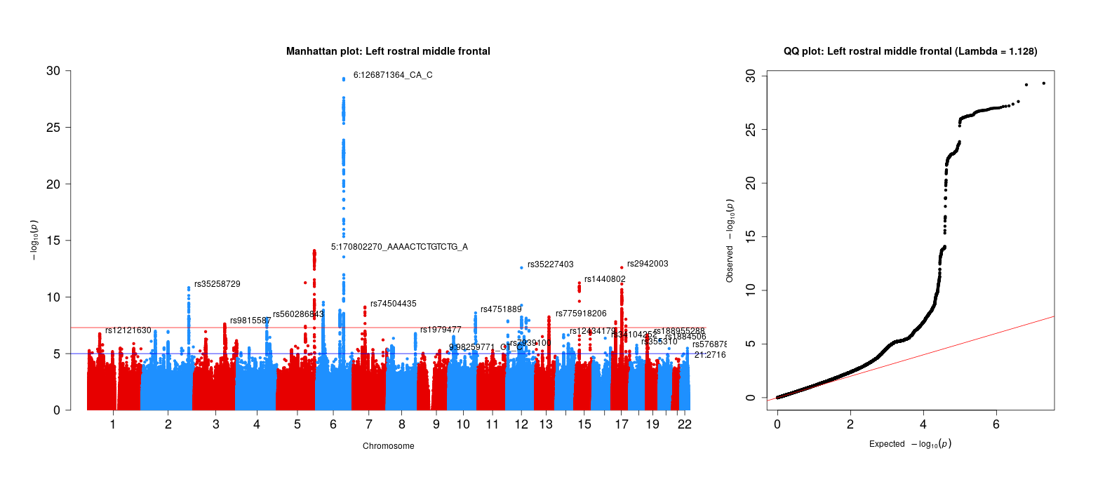
Left rostral middle frontal GWAS
![]()
By Anna Elisabeth Fürtjes
anna.furtjes@kcl.ac.uk