Genetic correlations

Author

Anna Elisabeth Furtjes

Published

June 6, 2025

Doi

10.1101/2024.11.06.622274

Genetic correlations in GenomicSEM

Munge

Code

library(devtools)
# install_github("GenomicSEM/GenomicSEM")
library(GenomicSEM)
library(stringr)
library(data.table)

#######################################################################
### MUNGE
#######################################################################
files <- list.files(pattern = "GWAS_brainAtrophy_")
#files <- files[grepl("males", files)]
hm3 <- "/eur_w_ld_chr/w_hm3.snplist"
maf.filter = 0.01
info.filter = 0.9

# cycle through each of the files
for(i in files){

    # read in file first
    file <- fread(i)
    # if it's residual or ratio score, we flip the effect sizes because that was also done throughout the rest of manuscript to harmonise the scores (higher score, more atrophy)
    if(grepl("ratio|resid", i)){
        file$BETA <- file$BETA * (-1)
    }
    # write temporarily because munge can't read in gz files
    fwrite(file, paste0("temp",i,".txt"), na = "NA", quote = F, sep = "\t", row.names = FALSE, col.names = TRUE)

    # isolate trait name
    trait.name = str_remove(i, "GWAS_brainAtrophy_")
    trait.name = str_remove(trait.name, "_N43110.gz")

    # munge this file
    munge(files = paste0("temp",i,".txt"), 
            trait.names = trait.name,
            hm3 = hm3, 
            maf.filter = maf.filter, 
            info.filter = info.filter,
            log.name = paste0(trait.name),
            column.names = list(SNP = "ID", 
                                A1 = "ALLELE1",
                                A2 = "ALLELE0", 
                                effect = "BETA", 
                                P = "P", 
                                N = "N"))
    # remove temp file again
    file.remove(paste0("temp",i,".txt"))
}

############################################################
#### Munging difficult sumstats
############################################################
library(devtools)
library(GenomicSEM)
library(stringr)
library(data.table)
library(tidyr)


setwd("/BrainAtrophy/data/GWASsumstats")

hm3 <- "/BrainAtrophy/eur_w_ld_chr/w_hm3.snplist"
maf.filter = 0.01
info.filter = 0.9

i=list.files(pattern = "CHARGE")
file <- fread(i, fill=TRUE)

# separate fused column
file <- separate(file, col = "N RSNUMBERS", into = c("N","RSNUMBER"), sep = " ")
# some rows are empty and the entry has shifted to to column V13
file$RSNUMBER <- ifelse(is.na(file$RSNUMBER), file$V13, file$RSNUMBER)
# problem with p-value column - rename
names(file)[grep("P-", names(file))] <- "P"

# write temporarily because munge can't read in gz files
fwrite(file, paste0("temp",i,".txt"), na = "NA", quote = F, sep = "\t", row.names = FALSE, col.names = TRUE)

# isolate trait name
trait.name = "ICV_Adams.et.al"

# munge this file
munge(files = paste0("temp",i,".txt"), 
        trait.names = trait.name,
        hm3 = hm3, 
        maf.filter = maf.filter, 
        info.filter = info.filter,
        log.name = paste0(trait.name),
        column.names = list(SNP = "RSNUMBER", 
                            A1 = "Allele1",
                            A2 = "Allele2", 
                            Z = "Zscore", 
                            P = "P", 
                            N = "Weight"))

# remove temp file again
file.remove(paste0("temp",i,".txt"))

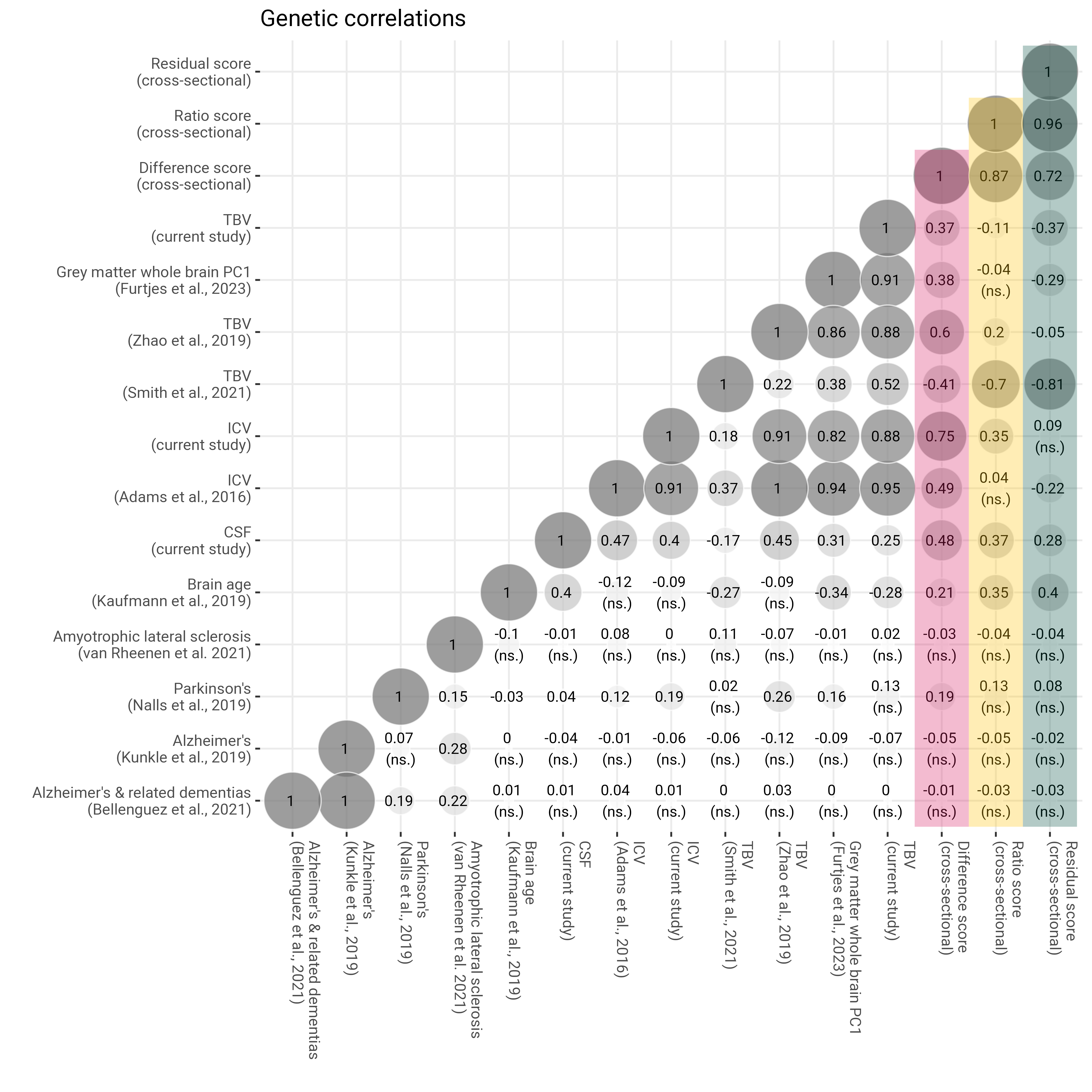
Genetic correlations

Code

#######################################################################
### LDSC
#######################################################################
library(devtools)
library(GenomicSEM)
library(stringr)

# vector of munged sumstats
traits <- list.files(pattern = ".sumstats.gz")
# remove log files
traits <- traits[!grepl(".log", traits)]
# remove BrainChange GWAS because they produce negative h2 estimate
traits = traits[!grepl("BrainChange", traits)]
# remove male and female specific sumstats
traits = traits[!grepl("males", traits)]
# remove SNP-by-age analyses
traits = traits[!grepl("SNPxage", traits)]

# trait.names
trait.names <- str_remove(traits, pattern = ".sumstats.gz")
# folder with ld scores
ld = "eur_w_ld_chr/"
# folder with ld weights
wld = "eur_w_ld_chr/"

# run ldsc
LDSCoutput <- ldsc(traits = traits, 
                    ld = ld, wld = wld, 
                    sample.prev = rep(NA, length(traits)),
                    population.prev = rep(NA, length(traits)),
                    trait.names = trait.names,
                    stand = T)

# dimnames
dimnames(LDSCoutput$S)[[1]] <- dimnames(LDSCoutput$S)[[2]]
dimnames(LDSCoutput$S_Stand)[[1]] <- dimnames(LDSCoutput$S)[[2]]
dimnames(LDSCoutput$S_Stand)[[2]] <- dimnames(LDSCoutput$S)[[2]]
dimnames(LDSCoutput$I)[[1]] <- dimnames(LDSCoutput$S)[[2]]
dimnames(LDSCoutput$I)[[2]] <- dimnames(LDSCoutput$S)[[2]]

save(LDSCoutput, file = "LDSCoutput_neurodegenrative.RData")
#save(LDSCoutput, file = "LDSCoutput_sexsplit.RData")

###########################################################################
#### Calculate associated matrix of Z statistics for this rG matrix
###########################################################################
library(gdata)
S_LD<-LDSCoutput$S

#pull V: the sampling covariance matrix
V_LD<-LDSCoutput$V

#standardize S [equivalent of cov2cor]
D=sqrt(diag(diag(S_LD)))
S_Stand=solve(D)%*%S_LD%*%solve(D)
rownames(S_Stand)<-rownames(S_LD)
colnames(S_Stand)<-colnames(S_Stand)

#obtain diagonals of the original V matrix and take their sqrt to get SE's
Dvcov<-sqrt(diag(V_LD))

#calculate the ratio of the rescaled and original S matrices
scaleO=as.vector(lowerTriangle((S_Stand/S_LD),diag=T))

## Make sure that if ratio in NaN (devision by zero) we put the zero back in
scaleO[is.nan(scaleO)] <- 0

#rescale the SEs by the same multiples that the S matrix was rescaled by
Dvcovl<-as.vector(Dvcov*t(scaleO))

#obtain the sampling correlation matrix by standardizing the original V matrix
Vcor<-cov2cor(V_LD)

#rescale the sampling correlation matrix by the appropriate diagonals
V_stand<-diag(Dvcovl)%*%Vcor%*%diag(Dvcovl)

#calculate SEs of rg
k<-nrow(LDSCoutput$S)
SE_stand<-matrix(0, k, k)
SE_stand[lower.tri(SE_stand,diag=TRUE)] <-sqrt(diag(V_stand))

#calculate Z of rg matrix
Z_cor<-S_Stand/SE_stand

Plot results (full sample)

Code

###########################################################################
#### Genetic correlation matrix
###########################################################################
### INCLUDE NEURODEGENERATIVE DISEASES

load("LDSCoutput_neurodegenrative.RData")

# pull out correlation matrix
cormat <- LDSCoutput$S_Stand

# re-roder
cormat = cormat[c("ALZ", "ALZ_2019", "PD", "ALS", "ICV_Adams.et.al", "TBV_Zhao.et.al", "TBV_Smith.et.al", "PC1_whole_brain_greymatter", "brainage", "ICVstand", "TBVstand", "CSFstand", "diff_stand", "ratio_stand", "resid_stand"), c("ALZ", "ALZ_2019", "PD", "ALS", "ICV_Adams.et.al", "TBV_Zhao.et.al", "TBV_Smith.et.al", "PC1_whole_brain_greymatter", "brainage", "ICVstand", "TBVstand", "CSFstand", "diff_stand", "ratio_stand", "resid_stand")]

# re-name
dimnames(cormat)[[1]] <-c("Alzheimer's & related dementias\n(Bellenguez et al., 2021)", "Alzheimer's\n(Kunkle et al., 2019)", "Parkinson's\n(Nalls et al., 2019)", "Amyotrophic lateral sclerosis\n(van Rheenen et al. 2021)", "ICV\n(Adams et al., 2016)", "TBV\n(Zhao et al., 2018)", "TBV\n(Smith et al., 2021)", "Grey matter whole brain PC1\n(Furtjes et al., 2023)", "Brain age\n(Kaufmann et al., 2019)","ICV", "TBV", "CSF", "Difference score\n(cross)", "Ratio score\n(cross)", "Residual score\n(cross)")
dimnames(cormat)[[2]] <-c("Alzheimer's & related dementias\n(Bellenguez et al., 2021)", "Alzheimer's\n(Kunkle et al., 2019)", "Parkinson's\n(Nalls et al., 2019)", "Amyotrophic lateral sclerosis\n(van Rheenen et al. 2021)", "ICV\n(Adams et al., 2016)", "TBV\n(Zhao et al., 2018)", "TBV\n(Smith et al., 2021)", "Grey matter whole brain PC1\n(Furtjes et al., 2023)", "Brain age\n(Kaufmann et al., 2019)","ICV", "TBV", "CSF", "Difference score\n(cross)", "Ratio score\n(cross)", "Residual score\n(cross)")

# define function to obtain lower triangle
  get_lower_tri<-function(cormat){
    cormat[upper.tri(cormat)] <- NA
    return(cormat)
  }

  # get correlation matrix for both samples together
  cor = get_lower_tri(cormat)
  # melt matrix
  melted = reshape2::melt(cor)
    # one value is > 1 which can happen sometimes
    melted$value[melted$value > 1.01] <- 1
    # get rounded value
  melted$value_round = round(melted$value, digit = 2)
  melted$distance0 = abs(melted$value)

    # for some reason one corr over 1 doesn't get colored
    melted$value <- ifelse(melted$value > 1, 1, melted$value)

    # pull out standard errors
    # SEs will be listed in the same order as they are listed in the genetic covariance matrix  
    r<-nrow(LDSCoutput$S)
    SE_Stand<-matrix(0, r, r)
    SE_Stand[lower.tri(SE_Stand,diag=TRUE)] <-sqrt(diag(LDSCoutput$V_Stand))
    dimnames(SE_Stand)<- dimnames(LDSCoutput$S)

    # re-roder
    SE_Stand = SE_Stand[c("ALZ","ALZ_2019","PD","ALS","ICV_Adams.et.al","TBV_Zhao.et.al", "TBV_Smith.et.al", "PC1_whole_brain_greymatter","brainage", "ICVstand", "TBVstand", "CSFstand", "diff_stand", "ratio_stand", "resid_stand"), c("ALZ","ALZ_2019","PD","ALS","ICV_Adams.et.al", "TBV_Zhao.et.al", "TBV_Smith.et.al", "PC1_whole_brain_greymatter","brainage", "ICVstand", "TBVstand", "CSFstand", "diff_stand", "ratio_stand", "resid_stand")]

    # re-name
    dimnames(SE_Stand)[[1]] <-c("Alzheimer's & related dementias\n(Bellenguez et al., 2021)", "Alzheimer's\n(Kunkle et al., 2019)", "Parkinson's\n(Nalls et al., 2019)", "Amyotrophic lateral sclerosis\n(van Rheenen et al. 2021)", "ICV\n(Adams et al., 2016)", "TBV\n(Zhao et al., 2018)", "TBV\n(Smith et al., 2021)", "Grey matter whole brain PC1\n(Furtjes et al., 2023)", "Brain age\n(Kaufmann et al., 2019)","ICV", "TBV", "CSF", "Difference score\n(cross)", "Ratio score\n(cross)", "Residual score\n(cross)")
    dimnames(SE_Stand)[[2]] <-c("Alzheimer's & related dementias\n(Bellenguez et al., 2021)", "Alzheimer's\n(Kunkle et al., 2019)", "Parkinson's\n(Nalls et al., 2019)", "Amyotrophic lateral sclerosis\n(van Rheenen et al. 2021)", "ICV\n(Adams et al., 2016)", "TBV\n(Zhao et al., 2018)", "TBV\n(Smith et al., 2021)", "Grey matter whole brain PC1\n(Furtjes et al., 2023)", "Brain age\n(Kaufmann et al., 2019)","ICV", "TBV", "CSF", "Difference score\n(cross)", "Ratio score\n(cross)", "Residual score\n(cross)")
    

    #melt data
    SEmelted <- reshape2::melt(SE_Stand)
    names(SEmelted)[grepl("value", names(SEmelted))] <- "SE"
    # merge with corr data
    both = merge(melted, SEmelted, by = c("Var1", "Var2"), all.x = T)
    # work out confidence intervals
    both$ci_u <- both$value + (1.96*both$SE)
    both$ci_l <- both$value - (1.96*both$SE)

    # get sig assocs
    both$sig <- ""
    both$sig[which(both$ci_u > 0 & both$ci_l < 0)] <- "\n(ns.)"
    both$sig[which(both$ci_u < 0 & both$ci_l > 0)] <- "\n(ns.)"
    both$sig[is.na(both$value)] <- NA
    both$value_round <- paste0(both$value_round, " ", both$sig)
    both$value_round[is.na(both$value)] <- NA
    #both$value_round[grep("NA", both$value_round)] <- str_remove(both$value_round[grep("NA", both$value_round)], pattern = " NA")

  # plot
  library(ggplot2)

  p = ggplot()+
    geom_point(data = both, aes(x = Var1, y = Var2, shape = value, fill = value, size = distance0), shape = 21, alpha = 0.7, colour = "white") +
    scale_fill_gradient2(low = "grey45", mid = "white", high = "grey45",limit = c(-1,1), space = "Lab" ,name="Correlation", guide = "legend")+
    scale_size_continuous(range = c(1, 15), guide = "none")+
    geom_text(data = both, aes(Var1, Var2, label = value_round), color = "black", size = 3)+
    geom_rect(aes(xmax = stage("Residual score\n(cross)", after_scale(xmax+0.5)), 
                    xmin = stage("Residual score\n(cross)", after_scale(xmin-0.5)), 
                    ymax = stage("Residual score\n(cross)", after_scale(ymax+0.5)), 
                    ymin = stage("Alzheimer's & related dementias\n(Bellenguez et al., 2021)", after_scale(ymin-0.5))), fill = "#004D40", alpha = 0.3)+
    geom_rect(aes(xmax = stage("Ratio score\n(cross)", after_scale(xmax+0.5)), 
                    xmin = stage("Ratio score\n(cross)", after_scale(xmin-0.5)), 
                    ymax = stage("Ratio score\n(cross)", after_scale(ymax+0.5)), 
                    ymin = stage("Alzheimer's & related dementias\n(Bellenguez et al., 2021)", after_scale(ymin-0.5))), fill = "#FFC107", alpha = 0.3)+
    geom_rect(aes(xmax = stage("Difference score\n(cross)", after_scale(xmax+0.5)), 
                    xmin = stage("Difference score\n(cross)", after_scale(xmin-0.5)), 
                    ymax = stage("Difference score\n(cross)", after_scale(ymax+0.5)), 
                    ymin = stage("Alzheimer's & related dementias\n(Bellenguez et al., 2021)", after_scale(ymin-0.5))), fill = "#D81B60", alpha = 0.3)+
    xlab("")+
    ylab("")+
    #scale_x_discrete(labels = axisNames)+
    #scale_y_discrete(labels = axisNames)+
    guides(fill = "none")+
    theme_bw()+
    theme(panel.border = element_blank(),
            axis.text.x = element_text(angle = 270, vjust = 0, hjust =0))+
    ggtitle("Genetic correlations")

ggsave("genetic_corr_neurodeg.png", plot = p, width = 22, height = 22, units = "cm", dpi = 600)

Plot sex-split correlations

Code

###########################################################################
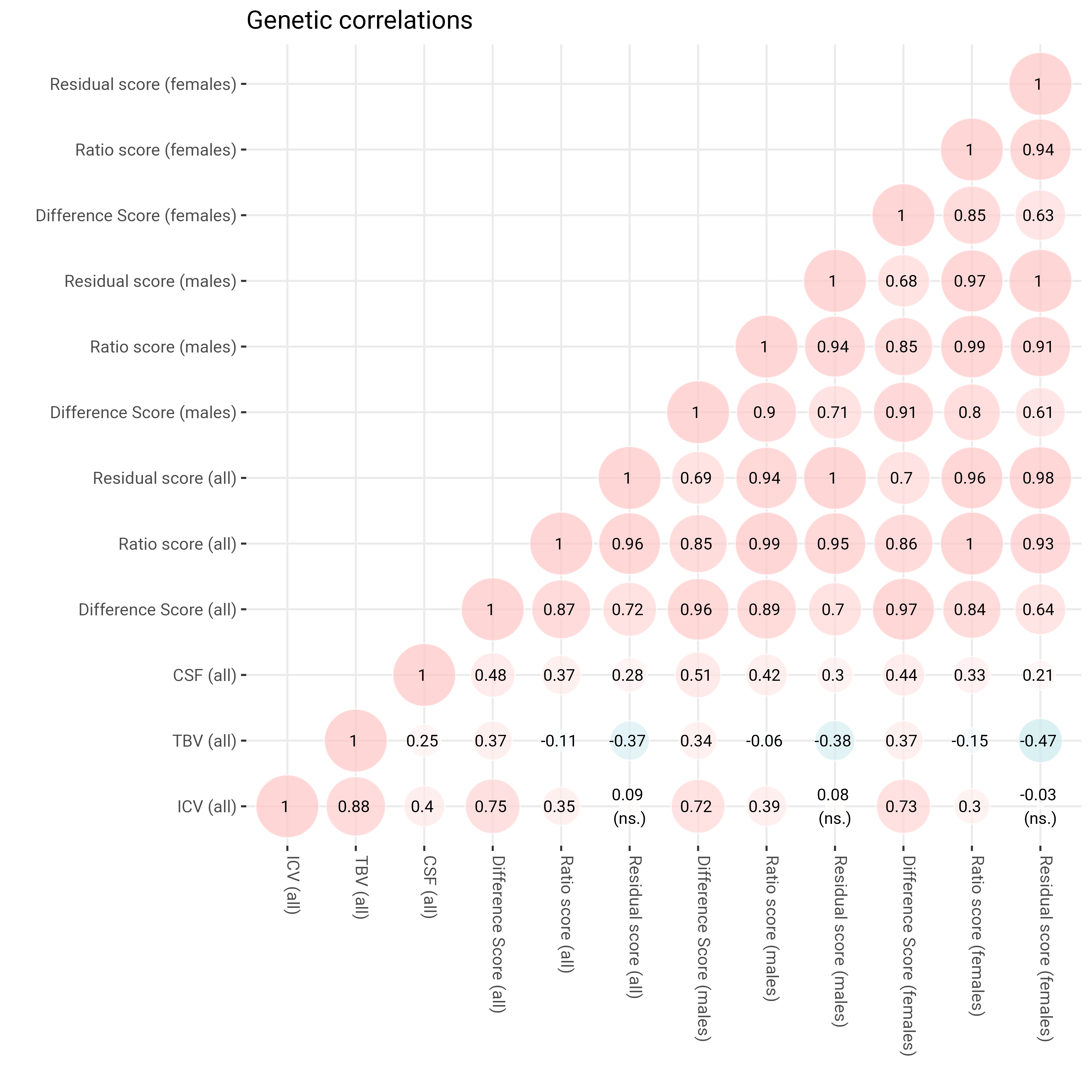
#### Genetic correlation matrix
#### Sex split
###########################################################################
load("LDSCoutput_sexsplit.RData")

# pull out correlation matrix
cormat <- LDSCoutput$S_Stand

# re-roder
cormat = cormat[c("ICVstand","TBVstand","CSFstand","diff_stand", "ratio_stand", "resid_stand", "diff_stand_males", "ratio_stand_males","resid_stand_males","diff_stand_females", "ratio_stand_females", "resid_stand_females"), c("ICVstand","TBVstand","CSFstand","diff_stand", "ratio_stand", "resid_stand", "diff_stand_males", "ratio_stand_males","resid_stand_males","diff_stand_females", "ratio_stand_females", "resid_stand_females")]

# re-name
dimnames(cormat)[[1]] <-c("ICV (all)","TBV (all)","CSF (all)","Difference Score (all)", "Ratio score (all)", "Residual score (all)", "Difference Score (males)", "Ratio score (males)","Residual score (males)","Difference Score (females)", "Ratio score (females)", "Residual score (females)")
dimnames(cormat)[[2]] <-c("ICV (all)","TBV (all)","CSF (all)","Difference Score (all)", "Ratio score (all)", "Residual score (all)", "Difference Score (males)", "Ratio score (males)","Residual score (males)","Difference Score (females)", "Ratio score (females)", "Residual score (females)")

# define function to obtain lower triangle
  get_lower_tri<-function(cormat){
    cormat[upper.tri(cormat)] <- NA
    return(cormat)
  }

  # get correlation matrix for both samples together
  cor = get_lower_tri(cormat)
  # melt matrix
  melted = reshape2::melt(cor)
    # one value is > 1 which can happen sometimes
    melted$value[melted$value > 1.01] <- 1
    # get rounded value
  melted$value_round = round(melted$value, digit = 2)
  melted$distance0 = abs(melted$value)

    # for some reason one corr over 1 doesn't get colored
    melted$value <- ifelse(melted$value > 1, 1, melted$value)

    # pull out standard errors
    # SEs will be listed in the same order as they are listed in the genetic covariance matrix  
    r<-nrow(LDSCoutput$S)
    SE_Stand<-matrix(0, r, r)
    SE_Stand[lower.tri(SE_Stand,diag=TRUE)] <-sqrt(diag(LDSCoutput$V_Stand))
    dimnames(SE_Stand)<- dimnames(LDSCoutput$S)

    # re-roder
    SE_Stand = SE_Stand[c("ICVstand","TBVstand","CSFstand","diff_stand", "ratio_stand", "resid_stand", "diff_stand_males", "ratio_stand_males","resid_stand_males","diff_stand_females", "ratio_stand_females", "resid_stand_females") ,c("ICVstand","TBVstand","CSFstand","diff_stand", "ratio_stand", "resid_stand", "diff_stand_males", "ratio_stand_males","resid_stand_males","diff_stand_females", "ratio_stand_females", "resid_stand_females")]

    # re-name
    dimnames(SE_Stand)[[1]] <-c("ICV (all)","TBV (all)","CSF (all)","Difference Score (all)", "Ratio score (all)", "Residual score (all)", "Difference Score (males)", "Ratio score (males)","Residual score (males)","Difference Score (females)", "Ratio score (females)", "Residual score (females)")
    dimnames(SE_Stand)[[2]] <-c("ICV (all)","TBV (all)","CSF (all)","Difference Score (all)", "Ratio score (all)", "Residual score (all)", "Difference Score (males)", "Ratio score (males)","Residual score (males)","Difference Score (females)", "Ratio score (females)", "Residual score (females)")
    

    #melt data
    SEmelted <- reshape2::melt(SE_Stand)
    names(SEmelted)[grepl("value", names(SEmelted))] <- "SE"
    # merge with corr data
    both = merge(melted, SEmelted, by = c("Var1", "Var2"), all.x = T)
    # work out confidence intervals
    both$ci_u <- both$value + (1.96*both$SE)
    both$ci_l <- both$value - (1.96*both$SE)

    # get sig assocs
    both$sig <- ""
    both$sig[which(both$ci_u > 0 & both$ci_l < 0)] <- "\n(ns.)"
    both$sig[which(both$ci_u < 0 & both$ci_l > 0)] <- "\n(ns.)"
    both$sig[is.na(both$value)] <- NA
    both$value_round <- paste0(both$value_round, " ", both$sig)
    both$value_round[is.na(both$value)] <- NA
    #both$value_round[grep("NA", both$value_round)] <- str_remove(both$value_round[grep("NA", both$value_round)], pattern = " NA")

  # plot
  library(ggplot2)

  p = ggplot()+
    geom_point(data = both, aes(x = Var1, y = Var2, shape = value, fill = value, size = distance0), shape = 21, alpha = 0.7, colour = "white") +
    scale_fill_gradient2(low = "#91D2D9", mid = "white", high = "#FFC4C4",limit = c(-1,1), space = "Lab" ,name="Correlation", guide = "legend")+
    scale_size_continuous(range = c(1, 15), guide = "none")+
    geom_text(data = both, aes(Var1, Var2, label = value_round), color = "black", size = 3)+
    xlab("")+
    ylab("")+
    #scale_x_discrete(labels = axisNames)+
    #scale_y_discrete(labels = axisNames)+
    guides(fill = "none")+
    theme_bw()+
    theme(panel.border = element_blank(),
            axis.text.x = element_text(angle = 270, vjust = 0, hjust =0))+
    ggtitle("Genetic correlations")

ggsave("genetic_corr_sexsplit.png", plot = p, width = 20, height = 20, units = "cm", dpi = 600)

GWAS-by-subtraction in GenomicSEM

Code

setwd(wd)
library(devtools)
library(GenomicSEM)

#### Step 2
traits <- c("TBVstand.sumstats.gz","ICVstand.sumstats.gz","resid_stand.sumstats.gz")
sample.prev <- rep(NA, length(traits))
population.prev <- rep(NA, length(traits))
ld<-"eur_w_ld_chr/"
wld <- "eur_w_ld_chr/"
trait.names<-c("TBV", "ICV", "resid")

LDSCoutput <- ldsc(traits = traits, 
                   sample.prev = sample.prev, 
                   population.prev = population.prev, 
                   ld=ld, 
                   wld=wld, 
                   trait.names=trait.names,
                    stand = T)


save(LDSCoutput, file="LDSCoutput_TBV_ICV.RData")

###### Step 3
load(file=paste0(wd, "/LDSCoutput_TBV_ICV.RData"))

# BaseICV is captured by both diff atrophy score and ICV
# Atrophy however should only be indicated by diff atrophy score and should be independent of ICV
model<-'
        BaseICV=~NA*TBV + ICV
        Atrophy=~NA*TBV
         
        # make sure all variances and covariances are captured by the latent factors
         Atrophy ~~ 1*Atrophy
         BaseICV ~~ 1*BaseICV
        # forcing atrophy and BaseICV to be uncorrelated
         Atrophy~~0*BaseICV

         ICV ~~ 0*TBV
         ICV ~~ 0*ICV
         TBV ~~ 0*TBV

        # add in resid to how correlated it is with Atrophy
        Atrophy ~~ resid
        BaseICV ~~ resid
'

# this is a fully saturated model (which is why no fit statistics are printed)
output<-usermodel(LDSCoutput,estimation="DWLS",model=model)

## Step 4
# files to prepare
files = c(paste0(GWASwd, "/GWAS_brainAtrophy_TBVstand_N43110.gz"), 
        paste0(GWASwd, "/GWAS_brainAtrophy_ICVstand_N43110.gz"))

file.exists(files)

ref = "reference.1000G.maf.0.005.txt.gz"
trait.names = c("TBV","ICV")
# SEs are not on a logistic scale
se.logit = c(F,F)
info.filter = 0.6
maf.filter = 0.01
#betas = c("BETA","BETA")

sumstats <- sumstats(files = files, 
                        ref = ref, 
                        trait.names = trait.names, 
                        se.logit = se.logit, 
                        info.filter = info.filter, 
                        maf.filter = maf.filter, 
                        #betas = betas,
                        OLS=c(T,T),
                        linprob=NULL,N=c(43110,43110), 
                        parallel = F)

save(sumstats, file="Sumstats_TBV_ICV.RData")

file.exists("Sumstats_TBV_ICV.RData")

SNP-level analysis

The script below makes it easier to parallelise SNP-level GWAS-by-subtraction analyses in GenomicSEM (make sure you change the model in the script when using this). Run this with: Rscript GWASbySubtractionPARALLEL.R --chr 3 --RData Sumstats_TBV_ICV.RData --LDSCout LDSCoutput_TBV_ICV.RData --outPath GWASbySubtraction

Code

#!/usr/bin/Rscript
# Run the 5th step of GWAS-by-subtraction to parallelise each chromosome 

if (!require("optparse")) install.packages("optparse", repos="https://cran.rstudio.com/")
suppressMessages(library("optparse"))


# SET OPTIONS
option_list = list(
  make_option("--chr", action = "store", default = NA, type = "character",
              help = "Chrosomome to be processed [required]"),
    make_option("--trait1", action = "store", default = NA, type = "character",
              help = "Trait 1 [required]"),
    make_option("--trait2", action = "store", default = NA, type = "character",
              help = "Trait 2 [required]"),
  make_option("--RData", action = "store", default = NA, type = "character",
              help = "RData containing cleaned sumstats [required]"),
    make_option("--LDSCout", action = "store", default = NA, type = "character",
              help = "LDSC output [required]"),
    make_option("--outPath", action = "store", default = NA, type = "character",
              help = "Output file name [required]")
)

opt = parse_args(OptionParser(option_list=option_list))

library(devtools)
library(GenomicSEM)

# FEEDBACK ON OPTIONS
print(Sys.time())
print(paste0("GWAS-by-subtraction CHR = ", opt$chr))

print(opt$RData)
print(paste0(opt$outPath,"/Atrophy_GWASbySubtraction", opt$chr,".RData"))

## Step 5
# load LDSC output
load(file=opt$LDSCout)

# load in RData file with cleaned SNP data
file = opt$RData
load(file)
# keep only one chromosome
sumstats = sumstats[which(sumstats$CHR == opt$chr),]

print(table(sumstats$CHR))

# SNP model
modelSNP<-'
        BaseICV=~NA*TBV + start(0.8)*ICV
        Atrophy=~NA*TBV
         
        # make sure all variances and covariances are captured by the latent factors
         Atrophy ~~ 1*Atrophy
         BaseICV ~~ 1*BaseICV
         ICV ~~ 0*TBV
         ICV ~~ 0*ICV
         TBV ~~ 0*TBV

        # forcing atrophy and BaseICV to be uncorrelated
         Atrophy~~0*BaseICV

        # add in SNP effect
        Atrophy ~ SNP
        BaseICV ~ SNP
        SNP ~~ SNP
'



#Run the Genomic SEM GWAS
outputGWAS<-userGWAS(covstruc=LDSCoutput,
                    SNPs=sumstats,
                    estimation="ML",
                    sub =c("Atrophy ~ SNP"),
                    Q_SNP = T,
                    smooth_check = T, 
                    parallel = T,
                    GC = "standard",
                    MPI = F,
                    fix_measurement = T,
                    model=modelSNP,
                    cores = 5,
                    toler = F, 
                    SNPSE = F) # printwarn = FALSE

save(outputGWAS, file=paste0(opt$outPath,"/Atrophy_GWASbySubtraction_", opt$chr,".RData"))


##### Run with 
# Rscript GWASbySubtractionPARALLEL.R --chr 3 --RData Sumstats_TBV_ICV.RData --LDSCout LDSCoutput_TBV_ICV.RData --outPath GWASbySubtraction