Code
library(ggplot2)
library(data.table)
library(ggpubr)
library(patchwork)Results produced by the code below are described in the manuscript under section:
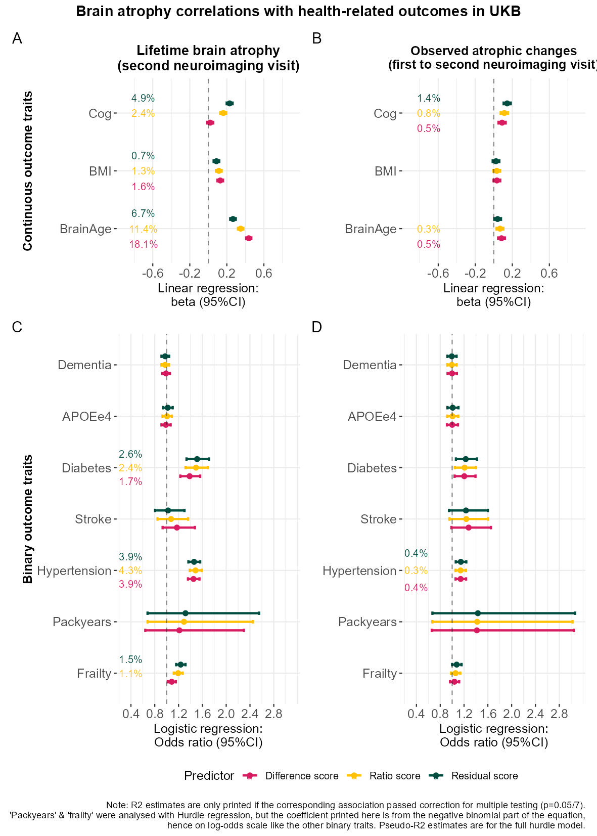
Measures of LBA predict brain atrophy rated by neuroradiological experts, as well as other ageing-related health traits such as frailty and cognitive ability.
The outcome traits were derived using code displayed in ‘Data preparation’: LBC: neuroimaging & phenotypic data; UKB: neuroimaging & phenotypic data.
library(ggplot2)
library(data.table)
library(ggpubr)
library(patchwork)This function calculates uni-variate associations across all outcomes in pheno and all predictors in neuro. The function detects whether traits are continuous, binary, or zero-inflated and runs the models accordingly with linear, logistic, or hurdle regression. The choice of model can be overwritten with the overwrite flag.
rawAssocAim3 = function(pheno = pheno,
                        neuro = neuro,
                        neuroVar = "resid_stand",
                        numOutcomeStand = FALSE,
                                    overwrite = NULL){

    # find ID column
    IDvar = names(pheno)[names(pheno) %in% names(neuro)]
    if(length(IDvar) == 0){warning("Pheno and neuro data do not share an ID column."); break}

    # keep neuro data from one time point only
    #neuro = neuro[which(neuro$wave == neuroWave),]
    # edit 8/4/2024: saved data for each wave individually so no need to subset anymore

    # merge the two data
    dat = merge(pheno, neuro, by = IDvar)

    # identify columns that can analysed with logit models
    bin = apply(pheno, 2, function(x){ all(na.omit(x) %in% 0:1)})
    binVar = attr(bin, "names")[bin]

    # identify columns that can be analysed with linear models
    # any variable where 50% or more of the entries are unique, I think it's safe to say its a continuous value
    num = apply(pheno, 2, function(x){ (length(unique(x))/length(x)) > 0.5 })
    numVar = names(pheno)[num]
    # this will however also pick up on IDvar
    numVar = numVar[numVar != IDvar]

    # standardise numeric variables if indicates
    if(isTRUE(numOutcomeStand)){
      dat[,numVar] = as.data.frame(lapply(dat[,numVar], scale))
    }else{message("You chose not to standardise your outcome variable. If that was an accident, use numOutcomeStand == TRUE")}

    # identify zero-inflated variables to be analysed with hurdle regression
    # if the mode in the data is represented in over 30% of the entries (and it's not binary), I think it's safe to say it's zero-inflated
    Mode = function(y){un = unique(y); un[which.max(tabulate(match(y, un)))]}
    mode = apply(pheno, 2, function(x){ sum(x == Mode(x), na.rm=T)/length(x) > 0.3 })
    modeVar = names(pheno)[mode]
    # remove binary variables from this category
    modeVar = modeVar[!modeVar %in% binVar]

    # if user specified to overwrite the categorisation of variables into num, bin and mode, here I assign the user specified data format
    if(!is.null(overwrite)){
        # remove assigned status from binVar, numVar, modeVar
        numVar = numVar[!numVar %in% overwrite$var]
        binVar = binVar[!binVar %in% overwrite$var]
        modeVar = modeVar[!modeVar %in% overwrite$var]

        # cycle through the rows in overwrite
        for(a in 1:nrow(overwrite)){
            if(overwrite$modelType[a] == "hurdle"){modeVar = append(modeVar, overwrite$var[a])}
            if(overwrite$modelType[a] == "logistic"){binVar = append(binVar, overwrite$var[a])}
            if(overwrite$modelType[a] == "linear"){numVar = append(numVar, overwrite$var[a])}
        }
    }

    # test if all variables have been assigned a category
    VarAvail = names(pheno)[which(names(pheno) != IDvar)]
    VarAssigned = c(binVar, numVar, modeVar)
    if(isFALSE(all(VarAvail %in% VarAssigned))){warning("It is not immediately obvious which category your variables belong to. Investigate and reformat to determine accurate statistical models! Alternatively, you can overwrite with the 'overwrite' command.")}

    # create object to hold results
    resNames = c("Outcome", "Predictor", "Stat.model", "beta", "std.error", "p.value", "R2_percent")
    results = data.frame(matrix(nrow = 0, ncol = length(resNames)))
    names(results) = resNames

    Index = nrow(results)
    ### calculate associations for linear models
    for(i in numVar){

      model = lm(paste0(i, " ~ ", neuroVar), data = dat)

      # store model info
      Index = Index+1
      results[Index,] = NA
      results$Outcome[Index] = i
      results$Predictor[Index] = neuroVar
      results$Stat.model[Index] = "Linear regression"
      results$beta[Index] = summary(model)$coefficients[2,1]
      results$std.error[Index] = summary(model)$coefficients[2,2]
      results$p.value[Index] = summary(model)$coefficients[2,4]
      results$R2_percent[Index] = summary(model)$r.squared*100
    }

    ### calculate logistic models
    for(i in binVar){
        # code prior to running this function should have made the binary variables factors

      model = glm(paste0(i, " ~ ", neuroVar), family = "binomial", data = dat)

      # store model info
      Index = Index+1
      results[Index,] = NA
      results$Outcome[Index] = i
      results$Predictor[Index] = neuroVar
      results$Stat.model[Index] = "Logistic regression"
      results$beta[Index] = summary(model)$coefficients[2,1]
      results$std.error[Index] = summary(model)$coefficients[2,2]
      results$p.value[Index] = summary(model)$coefficients[2,4]
      results$R2_percent[Index] = fmsb::NagelkerkeR2(model)$R2 *100

    }

    ## calculate hurdle models
    for(i in modeVar){
      # force variable to be inetger as the model will otherwise not run *made for count values)
      dat[,i] = as.integer(round(dat[,i]))

      model = pscl::hurdle(as.formula(paste0(i, " ~ ", neuroVar)), data = dat, dist="negbin")

      # store model info
      Index = Index+1
      results[Index,] = NA
      results$Outcome[Index] = i
      results$Predictor[Index] = neuroVar
      results$Stat.model[Index] = "Hurdle regression"
      results$beta[Index] = summary(model)$coefficient$zero[2,1]
      results$std.error[Index] = summary(model)$coefficient$zero[2,2]
      results$p.value[Index] = summary(model)$coefficient$zero[2,4]
      results$R2_percent[Index] = pscl::pR2(model)[5]*100

      message("Parameters for hurdle regression are zero hurdle model coefficient (binomial with logit link), but R2 is for both parts of the model.")
    }

    return(results)
}# read in LBC data
pheno = fread(paste0(wd, "/LBC1936_allPheno.txt"), data.table = F)
neuro = fread(paste0(wd, "/LBC1936_crossNeuroWave1.txt"), data.table = F)
# make sure binary variables are coded as factors because the function will otherwise not recognise it as factor
ColNames=c("dementia","APOEe4","diabetes","hypertension","Stroke")
pheno[ColNames] = lapply(pheno[ColNames], as.factor)
# make sure continuous variables are standardised (rawAssocAim3 deals with that)
#ColNames=c("iCog", "sCog", "iFrailty", "sFrailty", "iBMI", "sBMI", "BrainAge","ageMRI_w2")
#pheno[ColNames] = as.data.frame(scale(pheno[ColNames]))
# to ensure unified interpretation, I reverse code the ratio and residual score
neuro$resid_stand = neuro$resid_stand*(-1)
neuro$ratio_stand = neuro$ratio_stand*(-1)
# calculate raw associations for all atrophy scores
overwrite = data.frame(var = c("VisualAtrophyDeep", "VisualAtrophySuperficial"), modelType = c("linear", "linear"))
rawDiff = rawAssocAim3(pheno = pheno, neuro = neuro, neuroVar = "diff_stand", numOutcomeStand = TRUE, overwrite = overwrite)
rawRatio = rawAssocAim3(pheno = pheno, neuro = neuro, neuroVar = "ratio_stand", numOutcomeStand = TRUE, overwrite = overwrite)
rawResid = rawAssocAim3(pheno = pheno, neuro = neuro, neuroVar = "resid_stand", numOutcomeStand = TRUE, overwrite = overwrite)
raw2 = rbind(rawDiff, rawRatio, rawResid)pheno = fread(paste0(wd, "/LBC1936_allPheno.txt"), data.table = F)
neuro = fread(paste0(wd, "/LBC1936_crossNeuroWave4.txt"), data.table = F)
# make sure binary variables are coded as factors because the function will otherwise not recognise it as factor
ColNames=c("dementia","APOEe4","diabetes","hypertension","Stroke")
pheno[ColNames] = lapply(pheno[ColNames], as.factor)
# make sure continuous variables are standardised (rawAssocAim3 deals with that)
#ColNames=c("iCog", "sCog", "iFrailty", "sFrailty", "iBMI", "sBMI", "BrainAge","ageMRI_w2")
#pheno[ColNames] = as.data.frame(scale(pheno[ColNames]))
# to ensure unified interpretation, I reverse code the ratio and residual score
neuro$resid_stand = neuro$resid_stand*(-1)
neuro$ratio_stand = neuro$ratio_stand*(-1)
# calculate raw associations for all atrophy scores
overwrite = data.frame(var = c("VisualAtrophyDeep", "VisualAtrophySuperficial"), modelType = c("linear", "linear"))
rawDiff = rawAssocAim3(pheno = pheno, neuro = neuro, neuroVar = "diff_stand", numOutcomeStand = TRUE, overwrite = overwrite)
rawRatio = rawAssocAim3(pheno = pheno, neuro = neuro, neuroVar = "ratio_stand", numOutcomeStand = TRUE, overwrite = overwrite)
rawResid = rawAssocAim3(pheno = pheno, neuro = neuro, neuroVar = "resid_stand", numOutcomeStand = TRUE, overwrite = overwrite)
raw5 = rbind(rawDiff, rawRatio, rawResid)# read in LBC data
pheno = fread(paste0(wd, "/LBC1936_allPheno.txt"), data.table = F)
neuro = fread(paste0(wd, "/LBC1936_longTBVWaves2and5.txt"), data.table = F)
# make sure binary variables are coded as factors
ColNames=c("dementia","APOEe4","diabetes","hypertension","Stroke")
pheno[ColNames] = lapply(pheno[ColNames], as.factor)
# make sure continuous variables are standardised (rawAssocAim3 deals with that)
#ColNames=c("iCog", "sCog", "iFrailty", "sFrailty", "iBMI", "sBMI", "BrainAge","ageMRI_w2")
#pheno[ColNames] = as.data.frame(scale(pheno[ColNames]))
# to ensure unified interpretation, I reverse code the ratio and residual score
neuro$TBVresid_2to5_stand = neuro$TBVresid_2to5_stand*(-1)
neuro$TBVratio_5to2_stand = neuro$TBVratio_5to2_stand*(-1)
# calculate raw associations for all atrophy scores
overwrite = data.frame(var = c("VisualAtrophyDeep", "VisualAtrophySuperficial"), modelType = c("linear", "linear"))
rawDiff = rawAssocAim3(pheno = pheno, neuro = neuro, neuroVar = "TBVdiff_2to5_stand", numOutcomeStand = TRUE, overwrite = overwrite)
rawRatio = rawAssocAim3(pheno = pheno, neuro = neuro, neuroVar = "TBVratio_5to2_stand", numOutcomeStand = TRUE, overwrite = overwrite)
rawResid = rawAssocAim3(pheno = pheno, neuro = neuro, neuroVar = "TBVresid_2to5_stand", numOutcomeStand = TRUE, overwrite = overwrite)
rawObs = rbind(rawDiff, rawRatio, rawResid)# save cross data
raw2$wave = 2
raw5$wave = 5
raw = rbind(raw2, raw5)
raw$purpose = "Estimated Atrophy (cross-sectional)"
raw$purpose = "Estimated Atrophy (cross-sectional)"
rawObs$purpose = "Observed Atrophy (longitudinal)"
rawObs$wave = NA
save = rbind(raw, rawObs)
fwrite(save, file = paste0(wd, "/LBC1936_assocs_observed_vs_estimated_atrophy.txt"), col.names = T, row.names = F, quote = F, na = NA, sep = "\t")# read in LBC data
pheno = fread(paste0(wd, "/UKB_allPheno.txt"), data.table = F)
neuro = fread(paste0(wd, "/UKB_neuroNoLongProcess.txt"), data.table = F)
# get wave of interest
neuro = neuro[which(neuro$wave == 2),]
# edit:30/09/2024 (realised later that I hadn't cleaned the longitudinal data the same as the cross-sectional data, 10SD cutoff which some participants violate with the longitudinal data) - removed 6 participants
neuro <- neuro[which(neuro$TBVdiff_2to3_stand < 10),]
neuro <- neuro[which(neuro$TBVdiff_2to3_stand > (-10)),]
neuro <- neuro[which(neuro$TBVratio_3to2_stand < 10),]
neuro <- neuro[which(neuro$TBVratio_3to2_stand > (-10)),]
neuro <- neuro[which(neuro$TBVresid_2to3_stand < 10),]
neuro <- neuro[which(neuro$TBVresid_2to3_stand > (-10)),]
# to ensure unified interpretation, I reverse code the ratio and residual score
neuro$resid_stand = neuro$resid_stand*(-1)
neuro$ratio_stand = neuro$ratio_stand*(-1)
# make sure binary variables are coded as factors because the function will otherwise not recognise it as factor
ColNames=c("dementia","APOEe4","diabetes","hypertension","stroke")
pheno[ColNames] = lapply(pheno[ColNames], as.factor)
# make sure continuous variables are standardised (rawAssocAim3 deals with that)
#ColNames=c("cog", "BMI", "brainAge")
#pheno[ColNames] = as.data.frame(scale(pheno[ColNames]))
# calculate raw associations for all atrophy scores
overwrite = data.frame(var = c("packyears", "frailty"), modelType = c("hurdle", "hurdle")) # can overwrite with logistic of linear
rawDiff = rawAssocAim3(pheno = pheno, neuro = neuro, neuroVar = "diff_stand", numOutcomeStand = TRUE, overwrite = overwrite)
rawRatio = rawAssocAim3(pheno = pheno, neuro = neuro, neuroVar = "ratio_stand", numOutcomeStand = TRUE, overwrite = overwrite)
rawResid = rawAssocAim3(pheno = pheno, neuro = neuro, neuroVar = "resid_stand", numOutcomeStand = TRUE, overwrite = overwrite)
raw2 = rbind(rawDiff, rawRatio, rawResid)# read in data
pheno = fread(paste0(wd, "/UKB_allPheno.txt"), data.table = F)
neuro = fread(paste0(wd, "/UKB_neuroNoLongProcess.txt"), data.table = F)
# get wave of interest
neuro = neuro[which(neuro$wave == 3),]
# edit:30/09/2024 (realised later that I hadn't cleaned the longitudinal data the same as the cross-sectional data, 10SD cutoff which some participants violate with the longitudinal data) - removed 6 participants
neuro <- neuro[which(neuro$TBVdiff_2to3_stand < 10),]
neuro <- neuro[which(neuro$TBVdiff_2to3_stand > (-10)),]
neuro <- neuro[which(neuro$TBVratio_3to2_stand < 10),]
neuro <- neuro[which(neuro$TBVratio_3to2_stand > (-10)),]
neuro <- neuro[which(neuro$TBVresid_2to3_stand < 10),]
neuro <- neuro[which(neuro$TBVresid_2to3_stand > (-10)),]
# to ensure unified interpretation, I reverse code the ratio and residual score
neuro$resid_stand = neuro$resid_stand*(-1)
neuro$ratio_stand = neuro$ratio_stand*(-1)
# make sure binary variables are coded as factors because the function will otherwise not recognise it as factor
ColNames=c("dementia","APOEe4","diabetes","hypertension","stroke")
pheno[ColNames] = lapply(pheno[ColNames], as.factor)
# make sure continuous variables are standardised (rawAssocAim3 deals with that)
#ColNames=c("cog", "BMI", "brainAge")
#pheno[ColNames] = as.data.frame(scale(pheno[ColNames]))
# calculate raw associations for all atrophy scores
overwrite = data.frame(var = c("packyears", "frailty"), modelType = c("hurdle", "hurdle")) # can overwrite with logistic of linear
rawDiff = rawAssocAim3(pheno = pheno, neuro = neuro, neuroVar = "diff_stand", numOutcomeStand = TRUE, overwrite = overwrite)
rawRatio = rawAssocAim3(pheno = pheno, neuro = neuro, neuroVar = "ratio_stand", numOutcomeStand = TRUE, overwrite = overwrite)
rawResid = rawAssocAim3(pheno = pheno, neuro = neuro, neuroVar = "resid_stand", numOutcomeStand = TRUE, overwrite = overwrite)
raw5 = rbind(rawDiff, rawRatio, rawResid)# read in data
pheno = fread(paste0(wd, "/UKB_allPheno.txt"), data.table = F)
neuro = fread(paste0(wd, "/UKB_neuroNoLongProcess.txt"), data.table = F)
# shouldn't make a difference which wave we keep because long is saved double
neuro = neuro[which(neuro$wave == 2),]
# edit:30/09/2024 (realised later that I hadn't cleaned the longitudinal data the same as the cross-sectional data, 10SD cutoff which some participants violate with the longitudinal data) - removed 6 participants
neuro <- neuro[which(neuro$TBVdiff_2to3_stand < 10),]
neuro <- neuro[which(neuro$TBVdiff_2to3_stand > (-10)),]
neuro <- neuro[which(neuro$TBVratio_3to2_stand < 10),]
neuro <- neuro[which(neuro$TBVratio_3to2_stand > (-10)),]
neuro <- neuro[which(neuro$TBVresid_2to3_stand < 10),]
neuro <- neuro[which(neuro$TBVresid_2to3_stand > (-10)),]
# to ensure unified interpretation, I reverse code the ratio and residual score
neuro$TBVresid_2to3_stand = neuro$TBVresid_2to3_stand*(-1)
neuro$TBVratio_3to2_stand = neuro$TBVratio_3to2_stand*(-1)
# make sure binary variables are coded as factors because the function will otherwise not recognise it as factor
ColNames=c("dementia","APOEe4","diabetes","hypertension","stroke")
pheno[ColNames] = lapply(pheno[ColNames], as.factor)
# make sure continuous variables are standardised (rawAssocAim3 deals with that)
#ColNames=c("cog", "BMI", "brainAge")
#pheno[ColNames] = as.data.frame(scale(pheno[ColNames]))
# calculate raw associations for all atrophy scores
overwrite = data.frame(var = c("packyears", "frailty"), modelType = c("hurdle", "hurdle")) # can overwrite with logistic of linear
rawDiff = rawAssocAim3(pheno = pheno, neuro = neuro, neuroVar = "TBVdiff_2to3_stand", numOutcomeStand = TRUE, overwrite = overwrite)
rawRatio = rawAssocAim3(pheno = pheno, neuro = neuro, neuroVar = "TBVratio_3to2_stand", numOutcomeStand = TRUE, overwrite = overwrite)
rawResid = rawAssocAim3(pheno = pheno, neuro = neuro, neuroVar = "TBVresid_2to3_stand", numOutcomeStand = TRUE, overwrite = overwrite)
rawObs = rbind(rawDiff, rawRatio, rawResid)# save cross data
raw2$wave = 2
raw5$wave = 3
raw = rbind(raw2, raw5)
raw$purpose = "Estimated Atrophy (cross-sectional)"
raw$purpose = "Estimated Atrophy (cross-sectional)"
rawObs$purpose = "Observed Atrophy (longitudinal)"
rawObs$wave = NA
save = rbind(raw, rawObs)
fwrite(save, file = paste0(wd, "/UKB_assocs_observed_vs_estimated_atrophy.txt"), col.names = T, row.names = F, quote = F, na = NA, sep = "\t")# betas between atrophy scores and traits
setwd(wd)
file = list.files(pattern="LBC1936_assocs_observed_vs_estimated_atrophy")
assoc = fread(file)
# brain age phenotype is not intuitively interpretable:
# positive value should mean the participant has a healthier looking brain than expected given their age
# negative value should mean the participant has an unhealthier looking brain than expected
# Hence, here we just flip the assocs so that more LBA is associated with older brain age
assoc$beta[which(assoc$Outcome == "BrainAge")] <- assoc$beta[which(assoc$Outcome == "BrainAge")]*(-1)
# calculate lower and upper bounds of assoc
assoc$ci_l = assoc$beta - (1.96*assoc$std.error)
assoc$ci_u = assoc$beta + (1.96*assoc$std.error)
# because beta shouldn't exceed 1, and it makes the plots look ugly, I will artificially reduce those here
assoc$ci_l = ifelse(assoc$ci_l < -1.21, -1.21, assoc$ci_l)
assoc$ci_u = ifelse(assoc$ci_u > 1.21, 1.21, assoc$ci_u)
# make data frame for geom_label
assoc$label = paste0(round(assoc$R2_percent, digits = 1), "%")
# only print the label is correlation is significant
sigBonferroni = 0.05/length(unique(assoc$Outcome))
assoc$label[which(assoc$p.value > sigBonferroni)] = NA
######################################################################################
###### Continuous traits
######################################################################################
############## ESTIMATED ATROPHY
### first, only estimated atrophy
# only keep 'diff_stand', 'ratio_stand' or 'resid_stand'
estimated = assoc[grepl("diff_stand|ratio_stand|resid_stand",assoc$Predictor),]
# restrict to wave 5 (more atrophy)
estimated = estimated[grepl("5", estimated$wave),]
# restrict to continuous variables only
estimated = estimated[grepl("Linear", estimated$Stat.model)]
# c("iCog","sCog","Dementia","APOEe4","iFrailty","sFrailty","Diabetes","Stroke","Hypertension","iBMI","sBMI","BrainAge","Packyears")
# order phenotypes
estimated$Outcomes <- factor(estimated$Outcome,
levels=c("VisualAtrophySuperficial","VisualAtrophyDeep","iCog","sCog","iFrailty","sFrailty","iBMI","sBMI","BrainAge"),
labels = c("Visual atrophy\nrating\n (superficial)","Visual atrophy\nrating (deep)","iCog","sCog","iFrailty","sFrailty","iBMI","sBMI","BrainAge"),
ordered=T)
estLinear=ggplot(data=estimated, aes(y=Outcomes,x=beta),shape=3)+
xlim(-1.25, 1.25)+
geom_point(aes(col=Predictor),size=2,position=position_dodge(width=0.5))+
geom_errorbar(aes(xmin=ci_l, xmax=ci_u,col=Predictor), linewidth=1, width=.2,position=position_dodge(width=0.5))+
geom_vline(xintercept = 0, colour="grey10", alpha=0.5,linetype=2)+
geom_text(aes(y=Outcomes,x=-0.7, label = label, col=Predictor), size = 3.5, position=position_dodge(width=0.8))+
scale_y_discrete(limits = rev(levels(as.factor(estimated$Outcomes))))+ # reverse order of y-axis
scale_x_continuous(limits = c(-0.9, 0.9), breaks = seq(-1,1,by=0.4))+
theme_bw()+
ylab("Continuous outcome traits")+
xlab("Linear regression:\nbeta (95%CI)")+
ggtitle("Lifetime brain atrophy\nat age 82 years\n(wave 5)")+
scale_color_manual(labels = c("Difference score", "Ratio score", "Residual score"), values = c("#D81B60", "#FFC107", "#004D40")) +
theme(plot.title = element_text(face = "plain", size=17, hjust = 0.5))+ # add centred title
theme(text = element_text(size=12),
axis.text.x = element_text(size=12),#angle=45
axis.text.y = element_text(size=12),
axis.title.y = element_text(face="bold", colour='black', size=12),
axis.title.x = element_text(colour='black', size=12),
panel.border = element_blank(),
plot.title = element_text(face = "bold", colour='black', size=12))+
theme(legend.position="none")
### why is diff score always the other way? Sensible because larger diff score is worse, but smaller ratio score is worse
############## OBSERVED ATROPHY
### only keep longitudinal atrophy
observed = assoc[grepl("TBV",assoc$Predictor),]
# restrict to continuous variables only
observed = observed[grepl("Linear", observed$Stat.model)]
# order phenotypes
observed$Outcomes <- factor(observed$Outcome,
levels=c("VisualAtrophySuperficial","VisualAtrophyDeep","iCog","sCog","iFrailty","sFrailty","iBMI","sBMI","BrainAge"),
labels = c("Visual atrophy\nrating\n (superficial)","Visual atrophy\nrating (deep)","iCog","sCog","iFrailty","sFrailty","iBMI","sBMI","BrainAge"),
ordered=T)
obsLinear=ggplot(data=observed, aes(y=Outcomes,x=beta),shape=3)+
geom_point(aes(col=Predictor),size=2,position=position_dodge(width=0.5))+
geom_errorbar(aes(xmin=ci_l, xmax=ci_u,col=Predictor), linewidth=1, width=.2,position=position_dodge(width=0.5))+
geom_vline(xintercept = 0, colour="grey10", alpha=0.5,linetype=2)+
geom_text(aes(y=Outcomes,x=-0.7, label = label, col=Predictor), size = 3.5,position=position_dodge(width=0.8))+
scale_y_discrete(limits = rev(levels(as.factor(observed$Outcomes))))+ # reverse order of y-axis
scale_x_continuous(limits = c(-0.9, 0.9), breaks = seq(-1,1,by=0.4))+
theme_bw()+
ylab("ontinuous outcome traits")+
xlab("Linear regression:\nbeta (95%CI)")+
ggtitle("Observed atrophic changes\nbetween age 73 and 82\n(waves 2 to 5)")+
scale_color_manual(labels = c("Difference score", "Ratio score", "Residual score"), values = c("#D81B60", "#FFC107", "#004D40")) +
theme(plot.title = element_text(face = "plain", size=17, hjust = 0.5))+ # add centred title
theme(text = element_text(size=12),
axis.text.x = element_text(size=12),#angle=45
axis.text.y = element_text(size=12),
axis.title.y = element_blank(),
panel.border = element_blank(),
axis.title.x = element_text(colour='black', size=12),
plot.title = element_text(face = "bold", colour='black', size=12))+
theme(legend.position="none")
plot1 = estLinear +
obsLinear +
plot_layout(ncol = 2)
#plot_annotation(title = "Correlations with health-related outcomes in LBC",
#theme = theme(plot.title = element_text(face = "bold", colour = "black", size = 14, hjust = 0.5))) & theme(legend.position = 'bottom')
#ggpubr::annotate_figure(plot, top = text_grob("Correlations with health-related outcomes in LBC",
# color = "black", face = "bold", size = 14))
######################################################################################
###### Binary traits
######################################################################################
############## ESTIMATED ATROPHY
### first, only estimated atrophy
# only keep 'diff_stand', 'ratio_stand' or 'resid_stand'
estimated = assoc[grepl("diff_stand|ratio_stand|resid_stand",assoc$Predictor),]
# restrict to wave 5 (more atrophy)
estimated = estimated[grepl("5", estimated$wave),]
# restrict to continuous variables only
estimated = estimated[grepl("Logistic|Hurdle", estimated$Stat.model)]
# transform beta to OR
estimated$OR = exp(estimated$beta)
estimated$ORci_l = exp(estimated$beta - (1.96 * estimated$std.error))
estimated$ORci_u = exp(estimated$beta + (1.96 * estimated$std.error))
# display as log odds
estimated$logOdds = log(estimated$OR)
estimated$logOdds_ci_l = log(estimated$ORci_l)
estimated$logOdds_ci_u = log(estimated$ORci_u)
# order phenotypes
estimated$Outcomes <- factor(estimated$Outcome,
levels=c("dementia","APOEe4","diabetes","Stroke","hypertension","packyears"),
labels = c("Dementia","APOEe4","Diabetes","Stroke","Hypertension","Packyears"),
ordered=T)
estLog=ggplot(data=estimated, aes(y=Outcomes,x=OR),shape=3)+
xlim(0, 2.3)+
geom_point(aes(col=Predictor),size=2,position=position_dodge(width=0.5))+
geom_errorbar(aes(xmin=ORci_l, xmax=ORci_u,col=Predictor), linewidth=1, width=.2,position=position_dodge(width=0.5))+
geom_vline(xintercept = 1, colour="grey10", alpha=0.5,linetype=2)+
geom_text(aes(y=Outcomes,x=0.4, label = label, col=Predictor), size = 3.5,position=position_dodge(width=0.8))+
scale_y_discrete(limits = rev(levels(as.factor(estimated$Outcomes))))+ # reverse order of y-axis
scale_x_continuous(limits = c(0.3,3), breaks = seq(0,3,by=0.4))+
theme_bw()+
ylab("Binary outcome traits")+
xlab("Logistic regression:\nOdds ratio (95%CI)")+
#ggtitle("'Estimated' brain atrophy\n(at wave 5)")+
scale_color_manual(labels = c("Difference score", "Ratio score", "Residual score"), values = c("#D81B60", "#FFC107", "#004D40")) +
theme(plot.title = element_text(face = "plain", size=17, hjust = 0.5))+ # add centred title
theme(text = element_text(size=12),
axis.text.x = element_text(size=12),#angle=45
axis.text.y = element_text(size=12),
panel.border = element_blank(),
axis.title.y = element_text(face="bold", colour='black', size=12),
axis.title.x = element_text(colour='black', size=12),
plot.title = element_text(face = "bold", colour='black', size=13))+
theme(legend.position="none")
############## OBSERVED ATROPHY
### only keep longitudinal atrophy
observed = assoc[grepl("TBV",assoc$Predictor),]
# restrict to continuous variables only
observed = observed[grepl("Logistic|Hurdle", observed$Stat.model)]
# transform beta to OR
observed$OR = exp(observed$beta)
observed$ORci_l = exp(observed$beta - (1.96 * observed$std.error))
observed$ORci_u = exp(observed$beta + (1.96 * observed$std.error))
# order phenotypes
observed$Outcomes <- factor(observed$Outcome,
levels=c("dementia","APOEe4","diabetes","Stroke","hypertension","packyears"),
labels = c("Dementia","APOEe4","Diabetes","Stroke","Hypertension","Packyears"),
ordered=T)
obsLog=ggplot(data=observed, aes(y=Outcomes,x=OR),shape=3)+
geom_point(aes(col=Predictor),size=2,position=position_dodge(width=0.5))+
geom_errorbar(aes(xmin=ORci_l, xmax=ORci_u,col=Predictor), linewidth=1, width=.2,position=position_dodge(width=0.5))+
geom_vline(xintercept = 1, colour="grey10", alpha=0.5,linetype=2)+
geom_text(aes(y=Outcomes,x=0.4, label = label, col=Predictor), size = 3.5,position=position_dodge(width=1))+
scale_y_discrete(limits = rev(levels(as.factor(estimated$Outcomes))))+ # reverse order of y-axis
scale_x_continuous(limits = c(0,6.7), breaks = seq(0,6,by=1))+
theme_bw()+
ylab("Binary outcome traits")+
xlab("Logistic regression:\nOdds ratio (95%CI)")+
#ggtitle("'Observed' brain atrophy\n(wave 2 to 5)")+
scale_color_manual(labels = c("Difference score", "Ratio score", "Residual score"), values = c("#D81B60", "#FFC107", "#004D40")) +
theme(plot.title = element_text(face = "plain", size=17, hjust = 0.5))+ # add centred title
theme(text = element_text(size=12),
axis.text.x = element_text(size=12),#angle=45
axis.text.y = element_text(size=12),
panel.border = element_blank(),
axis.title.y = element_blank(),
axis.title.x = element_text(colour='black', size=12),
plot.title = element_text(face = "bold", colour='black', size=13),
legend.position = "bottom")
plot2 = estLog +
obsLog +
plot_layout(guides = "collect")
layout <- "
AB
AB
CD
"
plot <- estLinear + obsLinear + estLog + obsLog +
plot_layout(design = layout, guides = "collect")+
plot_annotation(title = "Brain atrophy associations with health-related outcomes in LBC",
caption = "Note: R2 estimates are only printed if the corresponding association passed correction for multiple testing (p=0.05/15).\n'Packyears' was analysed with Hurdle regression, but the coefficient printed here is from the negative binomial part of the equation,\nhence on log-odds scale like the other binary traits. Pseudo-R2 estimates are for the full hurdle model.",
tag_levels = "A",
theme = theme(legend.position = "bottom",plot.title = element_text(face = "bold", colour = "black", size = 14, hjust = 0.5)))
#ggsave(paste0(out,"phenotypic/LBC_assocs_cross_vs_long.jpg"), bg = "white",plot = plot, width = 20, height = 28, units = "cm", dpi = 300)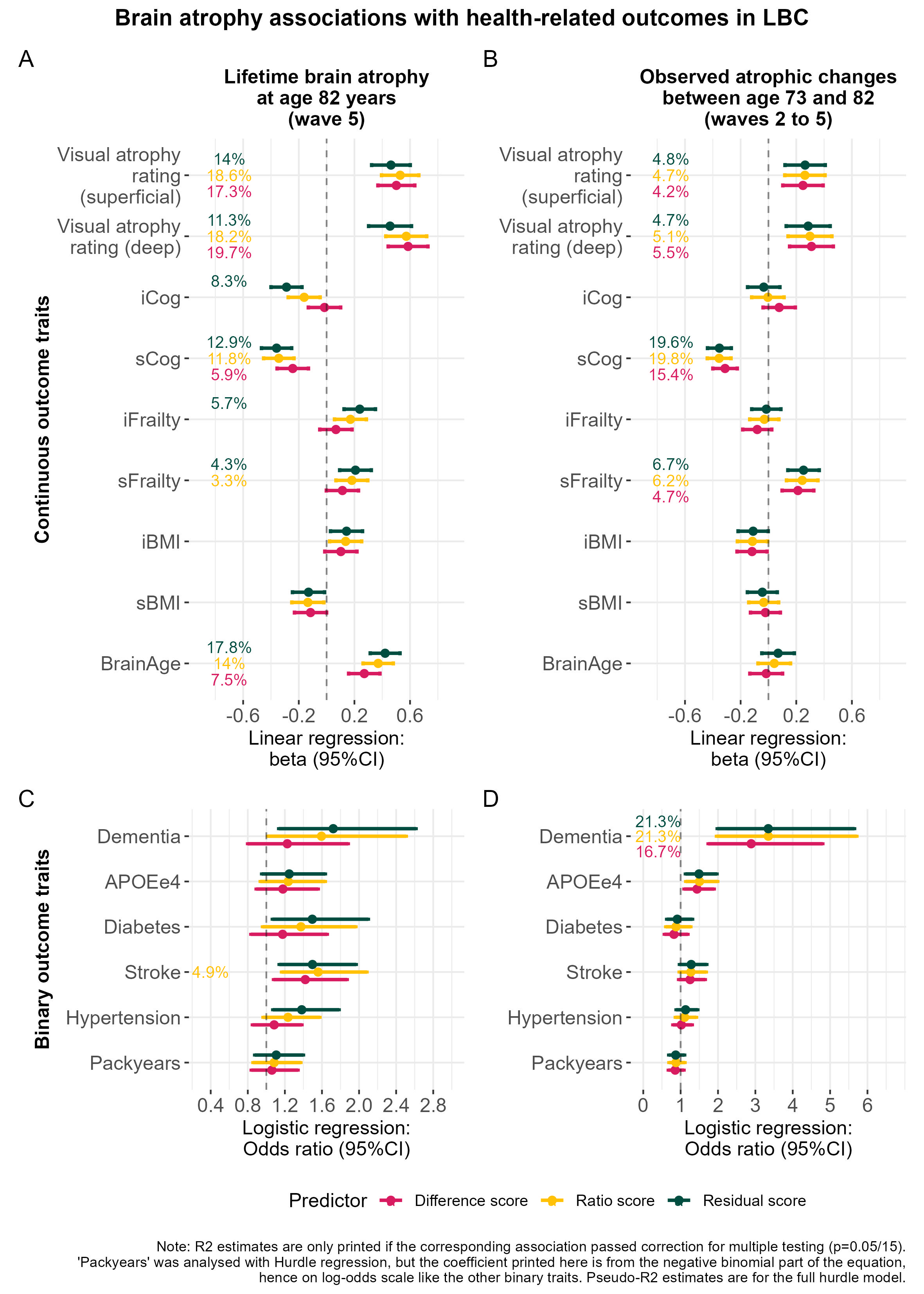
This plot is in Supplementary Plot 7.
# read in data
setwd(wd)
file = list.files(pattern="UKB_assocs_observed_vs_estimated_atrophy")
assoc = fread(file)

# brain age phenotype is not intuitively interpretable:
# positive value should mean the particpant has a healthier looking brain tthan expected given their age
# negative value should mean the participant has an unhealthier looking brain than expected
# Hence, here we just flip the assocs so that more LBA is associated with older brian age
assoc$beta[which(assoc$Outcome == "brainAge")] <- assoc$beta[which(assoc$Outcome == "brainAge")]*(-1)

# calculate lower and upper bounds of assoc
assoc$ci_l = assoc$beta - (1.96*assoc$std.error)
assoc$ci_u = assoc$beta + (1.96*assoc$std.error)

# because beta shouldn't exceed 1, and it makes the plots look ugly, I will artifically reduce those here
assoc$ci_l = ifelse(assoc$ci_l < -1.21, -1.21, assoc$ci_l)
assoc$ci_u = ifelse(assoc$ci_u > 1.21, 1.21, assoc$ci_u)

# make data frame for geom_label
assoc$label = paste0(round(assoc$R2_percent, digits = 1), "%")
# only print the label is correlation is significant
sigBonferroni = 0.05/length(unique(assoc$Outcome))
assoc$label[which(assoc$p.value > sigBonferroni)] = NA

######################################################################################
###### Continuous traits
######################################################################################
############## ESTIMATED ATROPHY
### first, only estimated atrophy
# only keep 'diff_stand', 'ratio_stand' or 'resid_stand'
estimated = assoc[grepl("diff_stand|ratio_stand|resid_stand",assoc$Predictor),]
# restrict to wave 3 (more atrophy)
estimated = estimated[grepl("3", estimated$wave),]
# restrict to continuous variables only
estimated = estimated[grepl("Linear", estimated$Stat.model)]

# order phenotypes
estimated$Outcomes <- factor(estimated$Outcome,
                             levels=c("cog","BMI","brainAge"),
                             labels = c("Cog","BMI","BrainAge"),
                             ordered=T)

estLinear=ggplot(data=estimated, aes(y=Outcomes,x=beta),shape=3)+
  xlim(-1.25, 1.25)+
  geom_point(aes(col=Predictor),size=2,position=position_dodge(width=0.5))+
  geom_errorbar(aes(xmin=ci_l, xmax=ci_u,col=Predictor), linewidth=1, width=.2,position=position_dodge(width=0.5))+
  geom_vline(xintercept = 0, colour="grey10", alpha=0.5,linetype=2)+
  geom_text(aes(y=Outcomes,x=-0.7, label = label, col=Predictor), size = 3.5, position=position_dodge(width=0.8))+
  scale_y_discrete(limits = rev(levels(as.factor(estimated$Outcomes))))+ # reverse order of y-axis
  scale_x_continuous(limits = c(-0.9, 0.9), breaks = seq(-1,1,by=0.4))+
    theme_bw()+
  ylab("Continuous outcome traits")+
  xlab("Linear regression:\nbeta (95%CI)")+
  ggtitle("Lifetime brain atrophy\n(second neuroimaging visit)")+
  scale_color_manual(labels = c("Difference score", "Ratio score", "Residual score"), values = c("#D81B60", "#FFC107", "#004D40")) +
  theme(plot.title = element_text(face = "plain", size=17, hjust = 0.5))+ # add centred title
  theme(text = element_text(size=12),
        axis.text.x = element_text(size=12),#angle=45
        axis.text.y = element_text(size=12),
        axis.title.y = element_text(face="bold", colour='black', size=12),
        axis.title.x = element_text(colour='black', size=12),
        panel.border = element_blank(),
        plot.title = element_text(face = "bold", colour='black', size=13))+
  theme(legend.position="none")

############## OBSERVED ATROPHY
### only keep longitudinal atrophy
observed = assoc[grepl("TBV",assoc$Predictor),]
# restrict to continuous variables only
observed = observed[grepl("Linear", observed$Stat.model)]

# order phenotypes
observed$Outcomes <- factor(observed$Outcome,
                             levels=c("cog","BMI","brainAge"),
                             labels = c("Cog","BMI","BrainAge"),
                             ordered=T)

obsLinear=ggplot(data=observed, aes(y=Outcomes,x=beta),shape=3)+
  geom_point(aes(col=Predictor),size=2,position=position_dodge(width=0.5))+
  geom_errorbar(aes(xmin=ci_l, xmax=ci_u,col=Predictor), linewidth=1, width=.2,position=position_dodge(width=0.5))+
  geom_vline(xintercept = 0, colour="grey10", alpha=0.5,linetype=2)+
  geom_text(aes(y=Outcomes,x=-0.7, label = label, col=Predictor), size = 3.5,position=position_dodge(width=0.8))+
    scale_y_discrete(limits = rev(levels(as.factor(observed$Outcomes))))+ # reverse order of y-axis
  scale_x_continuous(limits = c(-0.9, 0.9), breaks = seq(-1,1,by=0.4))+
  theme_bw()+
  ylab("ontinuous outcome traits")+
  xlab("Linear regression:\nbeta (95%CI)")+
  ggtitle("Observed atrophic changes\n(first to second neuroimaging visit)")+
  scale_color_manual(labels = c("Difference score", "Ratio score", "Residual score"), values = c("#D81B60", "#FFC107", "#004D40")) +
  theme(plot.title = element_text(face = "plain", size=17, hjust = 0.5))+ # add centred title
  theme(text = element_text(size=12),
        axis.text.x = element_text(size=12),#angle=45
        axis.text.y = element_text(size=12),
        axis.title.y = element_blank(),
        panel.border = element_blank(),
        axis.title.x = element_text(colour='black', size=12),
        plot.title = element_text(face = "bold", colour='black', size=12))+
  theme(legend.position="none")

######################################################################################
###### Binary traits
######################################################################################
############## ESTIMATED ATROPHY
### first, only estimated atrophy
# only keep 'diff_stand', 'ratio_stand' or 'resid_stand'
estimated = assoc[grepl("diff_stand|ratio_stand|resid_stand",assoc$Predictor),]
# restrict to visit 3 (more atrophy)
estimated = estimated[grepl("3", estimated$wave),]
# restrict to continuous variables only
estimated = estimated[grepl("Logistic|Hurdle", estimated$Stat.model)]

# transform beta to OR
estimated$OR = exp(estimated$beta)
estimated$ORci_l = exp(estimated$beta - (1.96 * estimated$std.error))
estimated$ORci_u = exp(estimated$beta + (1.96 * estimated$std.error))

# display as log odds
estimated$logOdds = log(estimated$OR)
estimated$logOdds_ci_l = log(estimated$ORci_l)
estimated$logOdds_ci_u = log(estimated$ORci_u)

# order phenotypes
estimated$Outcomes <- factor(estimated$Outcome,
                             levels=c("dementia","APOEe4","diabetes","stroke","hypertension","packyears","frailty"),
                             labels = c("Dementia","APOEe4","Diabetes","Stroke","Hypertension","Packyears","Frailty"),
                             ordered=T)

estLog=ggplot(data=estimated, aes(y=Outcomes,x=OR),shape=3)+
  xlim(0, 2.3)+
  geom_point(aes(col=Predictor),size=2,position=position_dodge(width=0.5))+
  geom_errorbar(aes(xmin=ORci_l, xmax=ORci_u,col=Predictor), linewidth=1, width=.2,position=position_dodge(width=0.5))+
  geom_vline(xintercept = 1, colour="grey10", alpha=0.5,linetype=2)+
  geom_text(aes(y=Outcomes,x=0.4, label = label, col=Predictor), size = 3.5,position=position_dodge(width=0.8))+
    scale_y_discrete(limits = rev(levels(as.factor(estimated$Outcomes))))+ # reverse order of y-axis
  scale_x_continuous(limits = c(0.3,3.1), breaks = seq(0,3,by=0.4))+
  theme_bw()+
  ylab("Binary outcome traits")+
  xlab("Logistic regression:\nOdds ratio (95%CI)")+
  #ggtitle("'Estimated' brain atrophy\n(at wave 5)")+
  scale_color_manual(labels = c("Difference score", "Ratio score", "Residual score"), values = c("#D81B60", "#FFC107", "#004D40")) +
  theme(plot.title = element_text(face = "plain", size=17, hjust = 0.5))+ # add centred title
  theme(text = element_text(size=12),
        axis.text.x = element_text(size=12),#angle=45
        axis.text.y = element_text(size=12),
        panel.border = element_blank(),
        axis.title.y = element_text(face="bold", colour='black', size=12),
        axis.title.x = element_text(colour='black', size=12),
        plot.title = element_text(face = "bold", colour='black', size=13))+
  theme(legend.position="none")

############## OBSERVED ATROPHY
### only keep longitudinal atrophy
observed = assoc[grepl("TBV",assoc$Predictor),]
# restrict to continuous variables only
observed = observed[grepl("Logistic|Hurdle", observed$Stat.model)]

# transform beta to OR
observed$OR = exp(observed$beta)
observed$ORci_l = exp(observed$beta - (1.96 * observed$std.error))
observed$ORci_u = exp(observed$beta + (1.96 * observed$std.error))

# order phenotypes
observed$Outcomes <- factor(observed$Outcome,
                             levels=c("dementia","APOEe4","diabetes","stroke","hypertension","packyears","frailty"),
                             labels = c("Dementia","APOEe4","Diabetes","Stroke","Hypertension","Packyears","Frailty"),
                             ordered=T)

obsLog=ggplot(data=observed, aes(y=Outcomes,x=OR),shape=3)+
  geom_point(aes(col=Predictor),size=2,position=position_dodge(width=0.5))+
  geom_errorbar(aes(xmin=ORci_l, xmax=ORci_u,col=Predictor), linewidth=1, width=.2,position=position_dodge(width=0.5))+
  geom_vline(xintercept = 1, colour="grey10", alpha=0.5,linetype=2)+
  geom_text(aes(y=Outcomes,x=0.4, label = label, col=Predictor), size = 3.5,position=position_dodge(width=1))+
  scale_y_discrete(limits = rev(levels(as.factor(estimated$Outcomes))))+ # reverse order of y-axis
  scale_x_continuous(limits = c(0.3,3.1), breaks = seq(0,3,by=0.4))+
  theme_bw()+
  ylab("Binary outcome traits")+
  xlab("Logistic regression:\nOdds ratio (95%CI)")+
  #ggtitle("'Observed' brain atrophy\n(wave 2 to 5)")+
  scale_color_manual(labels = c("Difference score", "Ratio score", "Residual score"), values = c("#D81B60", "#FFC107", "#004D40")) +
  theme(plot.title = element_text(face = "plain", size=17, hjust = 0.5))+ # add centred title
  theme(text = element_text(size=12),
        axis.text.x = element_text(size=12),#angle=45
        axis.text.y = element_text(size=12),
        panel.border = element_blank(),
        axis.title.y = element_blank(),
        axis.title.x = element_text(colour='black', size=12),
        plot.title = element_text(face = "bold", colour='black', size=13),
        legend.position = "bottom")

# plot all together
layout <- "
AB
CD
CD
"

plot <- estLinear + obsLinear + estLog + obsLog +
                    plot_layout(design = layout,guides = "collect")+
                    plot_annotation(title = "Brain atrophy correlations with health-related outcomes in UKB",
                  caption = "Note: R2 estimates are only printed if the corresponding association passed correction for multiple testing (p=0.05/7).\n'Packyears' & 'frailty' were analysed with Hurdle regression, but the coefficient printed here is from the negative binomial part of the equation,\nhence on log-odds scale like the other binary traits. Pseudo-R2 estimates are for the full hurdle model.",
                    tag_levels = "A",
                    theme = theme(legend.position = "bottom",plot.title = element_text(face = "bold", colour = "black", size = 14, hjust = 0.5)))

ggsave(paste0(out,"phenotypic/UKB_assocs_cross_vs_long.jpg"), bg = "white",plot = plot, width = 20, height = 28, units = "cm", dpi = 150)