Generation Scotland Subsample (STRADL)

---

Load packages

Code

library(data.table)
library(ggplot2)
library(ggpubr)

The STRADL data was kindly provided by Joanna Moodie where TBV and ICV had already been extracted.

Extract lifetime brain atrophy variables

Code

# add in STRADL
STRADL = fread(paste0(STRADLdir, "/", list.files(path = STRADLdir, pattern = "STRADL")))

names(STRADL) = c("ID", "Age", "Sex", "TBV", "ICV")

# convert mm3 estimates to more intuitive cm3 estimates
STRADL$ICV = STRADL$ICV/1000
STRADL$TBV = STRADL$TBV/1000

# estimate brain atrophy from single MRI scan
STRADL$diff = STRADL$ICV - STRADL$TBV
STRADL$ratio = STRADL$TBV / STRADL$ICV

# remove participants with zero estimates for TBV and ICV (11 participants)
STRADL = STRADL[STRADL$TBV != 0,]
STRADL = STRADL[STRADL$ICV != 0,]


# remove participants where ICV is smaller than TBV (excluding 45 participants)
STRADL = STRADL[which(STRADL$diff > 0),]

model <- lm(TBV ~ ICV, data = STRADL)
STRADL$resid = resid(model)

# standardise variables
STRADL$diff_stand = as.vector(scale(STRADL$diff))
STRADL$ratio_stand = as.vector(scale(STRADL$ratio))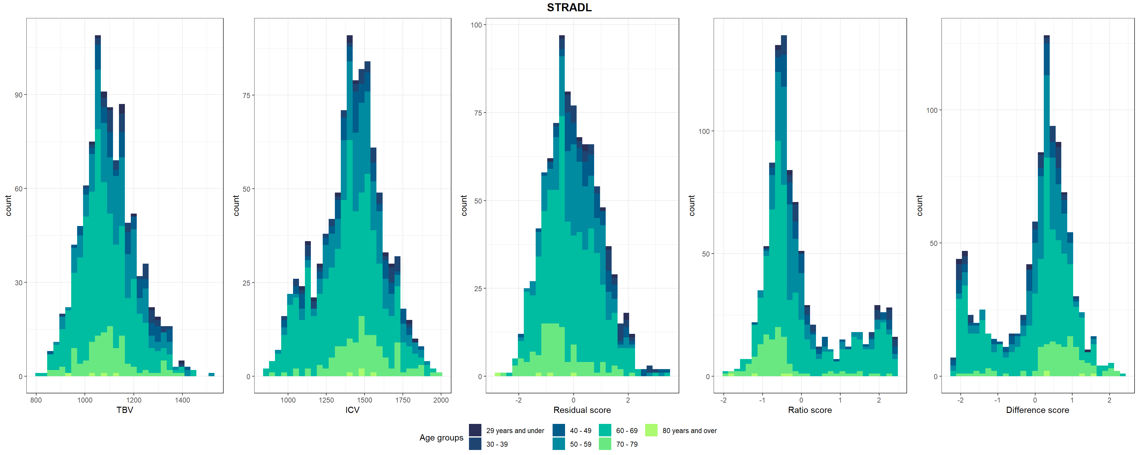
STRADL$resid_stand = as.vector(scale(STRADL$resid))

Plot distributions colored by age

Shown in Supplementary Figure 3: Distributions of TBV, ICV, and lifetime brain atrophy estimated with the residual, ratio, and difference method. Histograms are coloured by age groups.

Code

####################################################
# make age groups
STRADL$Age_group <- NA
STRADL$Age_group[STRADL$Age < 30] <- "29 years and under"
STRADL$Age_group[STRADL$Age >= 30 & STRADL$Age < 40] <- "30 - 39"
STRADL$Age_group[STRADL$Age >= 40 & STRADL$Age < 50] <- "40 - 49"
STRADL$Age_group[STRADL$Age >= 50 & STRADL$Age < 60] <- "50 - 59"
STRADL$Age_group[STRADL$Age >= 60 & STRADL$Age < 70] <- "60 - 69"
STRADL$Age_group[STRADL$Age >= 70 & STRADL$Age < 80] <- "70 - 79"
STRADL$Age_group[STRADL$Age >= 80] <- "80 years and over"

p1=ggplot(STRADL, aes(x=TBV, fill=Age_group)) +
  geom_histogram()+
  scale_fill_manual("Age groups", values = c("#292f56", "#1e4572", "#005c8b", "#008ba0", "#00bca1","#69e882", "#acfa70"))+
  xlab("TBV")+
  theme_bw()

p2=ggplot(STRADL, aes(x=ICV, fill=Age_group)) +
  geom_histogram()+
  scale_fill_manual("Age groups", values = c("#292f56", "#1e4572", "#005c8b", "#008ba0", "#00bca1","#69e882", "#acfa70"))+
  xlab("ICV")+
  theme_bw()

p3=ggplot(STRADL, aes(x=resid_stand, fill=Age_group)) +
  geom_histogram()+
  scale_fill_manual("Age groups", values = c("#292f56", "#1e4572", "#005c8b", "#008ba0", "#00bca1","#69e882", "#acfa70"))+
  xlab("Residual score")+
  theme_bw()

p4=ggplot(STRADL, aes(x=ratio_stand, fill=Age_group)) +
  geom_histogram()+
  scale_fill_manual("Age groups", values = c("#292f56", "#1e4572", "#005c8b", "#008ba0", "#00bca1","#69e882", "#acfa70"))+
  xlab("Ratio score")+
  theme_bw()

p5=ggplot(STRADL, aes(x=diff_stand, fill=Age_group)) +
  geom_histogram()+
  scale_fill_manual("Age groups", values = c("#292f56", "#1e4572", "#005c8b", "#008ba0", "#00bca1","#69e882", "#acfa70"))+
  xlab("Difference score")+
  theme_bw()

pSTRADL <- ggarrange(p1,p2,p3,p4,p5, nrow = 1, common.legend = T, legend = "bottom")

# add title
pSTRADL <- annotate_figure(pSTRADL, top = text_grob("STRADL",face = "bold", size = 14))

#ggsave(paste0(out,"phenotypic/STRADL_disttributions.jpg"), bg = "white",plot = pSTRADL, width = 30, height = 10, units = "cm", dpi = 300)
pSTRADL