MRi-Share sample

Author

Anna Elisabeth Furtjes

Published

June 6, 2025

Doi

10.1101/2024.11.06.622274

Load packages

Code

library(data.table)
library(ggplot2)
library(ggpubr)

Global measures from the MRi-Share sample can be freely downloaded online.

Read in data

Code

# read in MRi-Share
Share = fread(paste0(out, "/MRiShare_global_IDPs_BSAF2021.csv"))
Share$TBV = Share$SPM_GM_Volume + Share$SPM_WM_Volume
Share = Share[,c("ID", "Age", "Sex", "eTIV", "TBV")]
names(Share) = c("ID", "Age", "Sex", "ICV", "TBV")

# convert mm3 estimates to more intuitive cm3 estimates
Share$ICV = Share$ICV/1000
Share$TBV = Share$TBV/1000

# estimate brain atrophy from single MRI scan
Share$diff = Share$ICV - Share$TBV
Share$ratio = Share$TBV / Share$ICV

model <- lm(TBV ~ ICV, data = Share)
Share$resid = resid(model)

# save intercept value from the regression
Shareintercept = summary(model)$coefficients[1,1]

# standardise variables
Share$diff_stand = as.vector(scale(Share$diff))
Share$ratio_stand = as.vector(scale(Share$ratio))
Share$resid_stand = as.vector(scale(Share$resid))

# sanity check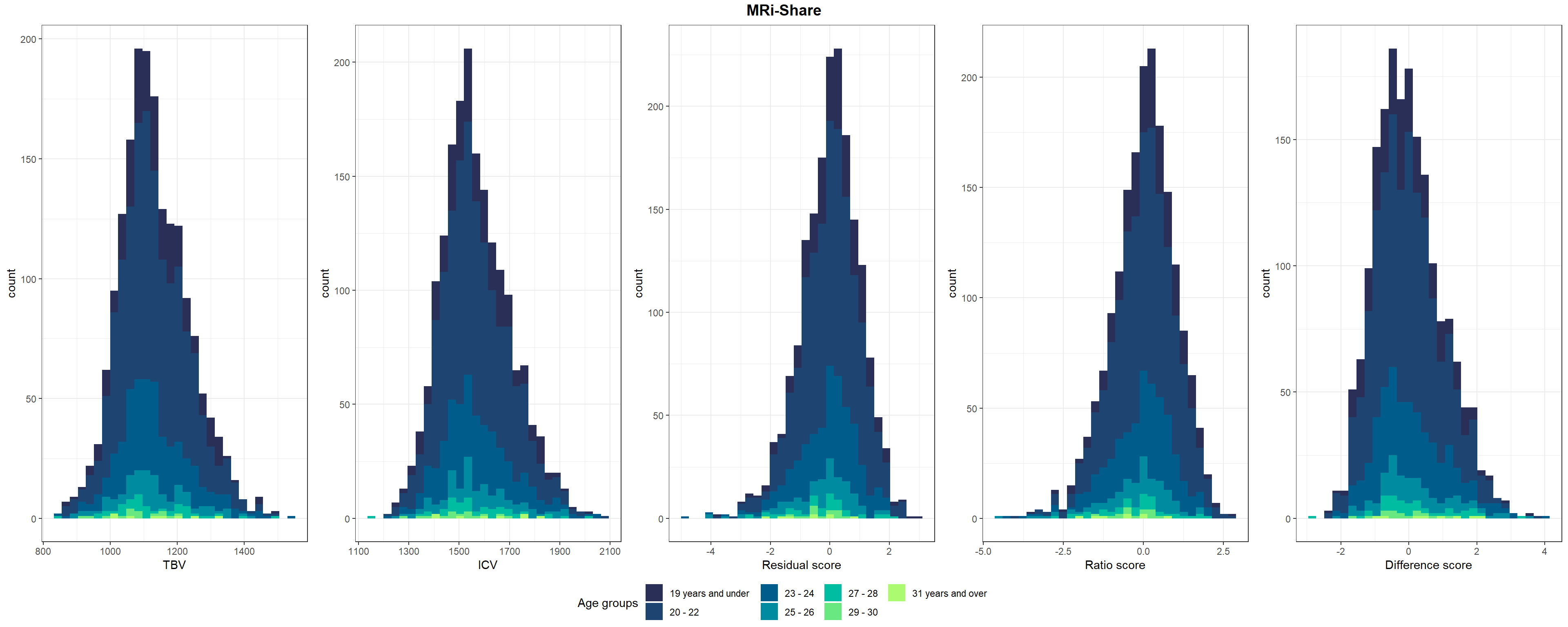
#sum((Share$diff < 0))

Plot distributions colored by age

Shown in Supplementary Figure 3: Distributions of TBV, ICV, and lifetime brain atrophy estimated with the residual, ratio, and difference method. Histograms are coloured by age groups.

Code

# make age groups
Share$Age_group <- NA
Share$Age_group[Share$Age < 20] <- "19 years and under"
Share$Age_group[Share$Age >= 20 & Share$Age < 23] <- "20 - 22"
Share$Age_group[Share$Age >= 23 & Share$Age < 25] <- "23 - 24"
Share$Age_group[Share$Age >= 25 & Share$Age < 27] <- "25 - 26"
Share$Age_group[Share$Age >= 27 & Share$Age < 29] <- "27 - 28"
Share$Age_group[Share$Age >= 29 & Share$Age < 31] <- "29 - 30"
Share$Age_group[Share$Age >= 31] <- "31 years and over"

p1=ggplot(Share, aes(x=TBV, fill=Age_group)) +
  geom_histogram()+
  scale_fill_manual("Age groups", values = c("#292f56", "#1e4572", "#005c8b", "#008ba0", "#00bca1","#69e882", "#acfa70"))+
  xlab("TBV")+
  theme_bw()

p2=ggplot(Share, aes(x=ICV, fill=Age_group)) +
  geom_histogram()+
  scale_fill_manual("Age groups", values = c("#292f56", "#1e4572", "#005c8b", "#008ba0", "#00bca1","#69e882", "#acfa70"))+
  xlab("ICV")+
  theme_bw()

p3=ggplot(Share, aes(x=resid_stand, fill=Age_group)) +
  geom_histogram()+
  scale_fill_manual("Age groups", values = c("#292f56", "#1e4572", "#005c8b", "#008ba0", "#00bca1","#69e882", "#acfa70"))+
  xlab("Residual score")+
  theme_bw()

p4=ggplot(Share, aes(x=ratio_stand, fill=Age_group)) +
  geom_histogram()+
  scale_fill_manual("Age groups", values = c("#292f56", "#1e4572", "#005c8b", "#008ba0", "#00bca1","#69e882", "#acfa70"))+
  xlab("Ratio score")+
  theme_bw()

p5=ggplot(Share, aes(x=diff_stand, fill=Age_group)) +
  geom_histogram()+
  scale_fill_manual("Age groups", values = c("#292f56", "#1e4572", "#005c8b", "#008ba0", "#00bca1","#69e882", "#acfa70"))+
  xlab("Difference score")+
  theme_bw()

pShare <- ggarrange(p1,p2,p3,p4,p5, nrow = 1, common.legend = T, legend = "bottom")
# add title
pShare <- annotate_figure(pShare, top = text_grob("MRi-Share",face = "bold", size = 14))

#ggsave(paste0(out,"phenotypic/Share_disttributions.jpg"), bg = "white",plot = pShare, width = 30, height = 10, units = "cm", dpi = 300)
pShare