Human Connectome Project

---

Load packages

Code

library(data.table)
library(ggplot2)
library(stringr)
library(ggpubr)
library(cowplot)
library(dplyr)

Read in and format the data

Code

HCPcov = fread(paste0(HCPdir,list.files(path = HCPdir, pattern = "unrestricted_annafurtjes")))
HCPcov = HCPcov[,c("Subject", "Release", "Acquisition","fMRI_3T_ReconVrs")]

HCP = fread(paste0(HCPdir,"unrestricted_hcp_freesurfer.csv"))
HCP = HCP[,c("Subject", "Gender", "FS_InterCranial_Vol", "FS_BrainSeg_Vol_No_Vent")]

HCP = merge(HCP, HCPcov, by = "Subject")

HCPage = fread(paste0(HCPdir, "RESTRICTED_annafurtjes_12_14_2023_4_18_2.csv"))
HCPage = HCPage[,c("Subject","Age_in_Yrs", "Family_ID")]

HCP = merge(HCP, HCPage, by ="Subject")
names(HCP) = c("ID", "Sex", "ICV", "TBV", "Release", "Acquisition","fMRI_3T_ReconVrs", "Age", "Family_ID")

# convert mm3 estimates to more intuitive cm3 estimates
HCP$ICV = HCP$ICV/1000
HCP$TBV = HCP$TBV/1000

# calculate atrophy scores
HCP$diff = HCP$ICV - HCP$TBV
HCP$ratio = HCP$TBV / HCP$ICV

# delete those from data 
HCP=HCP[-which(HCP$diff < 0),]

# estimate residual model
model <- lm(TBV ~ ICV, data = HCP)
HCP$resid = as.vector(resid(model, na.rm=T))

# standardise variables
HCP$diff_stand = as.vector(scale(HCP$diff))
HCP$ratio_stand = as.vector(scale(HCP$ratio))
HCP$resid_stand = as.vector(scale(HCP$resid))

Age correlations in the full sample

It is contrary to our expectation that ICV gets so much larger with younger age - cohort effect?

• Much stronger correlation between younger age and ICV than there should be (N = 1103)

• This explains why the atrophy scores with dependence of baseline levels are also strongly affected by age

• The only score that is independent of baseline levels - i.e., residual score - has no association with age

Code

corICV = ggplot(data = HCP, aes(x = ICV, y = Age))+
  geom_point(alpha = 0.2)+
  theme_bw()+
  geom_smooth(method='lm')+
  stat_cor(method = "pearson",color ="blue")+
  ylab("Age in years")+
  theme(panel.border = element_blank())

corTBV = ggplot(data = HCP, aes(x = TBV, y = Age))+
  geom_point(alpha = 0.2)+
  theme_bw()+
  geom_smooth(method='lm')+
  stat_cor(method = "pearson",color ="blue")+
  ylab("Age in years")+
  theme(panel.border = element_blank())

cordiff = ggplot(data = HCP, aes(x = diff, y = Age))+
  geom_point(alpha = 0.2)+
  theme_bw()+
  geom_smooth(method='lm')+
  stat_cor(method = "pearson",color ="blue")+
  ylab("Age in years")+
  xlab("Difference score")+
  theme(panel.border = element_blank())

corratio = ggplot(data = HCP, aes(x = ratio, y = Age))+
  geom_point(alpha = 0.2)+
  theme_bw()+
  geom_smooth(method='lm')+
  stat_cor(method = "pearson",color ="blue")+
  ylab("Age in years")+
  xlab("Ratio score")+
  theme(panel.border = element_blank())

corresid = ggplot(data = HCP, aes(x = resid, y = Age))+
  geom_point(alpha = 0.2)+
  theme_bw()+
  geom_smooth(method='lm')+
  stat_cor(method = "pearson",color ="blue")+
  ylab("Age in years")+
  xlab("Residual score")+
  theme(panel.border = element_blank())

ggarrange(corICV, corTBV, cordiff, corratio, corresid, common.legend=T, legend = "bottom")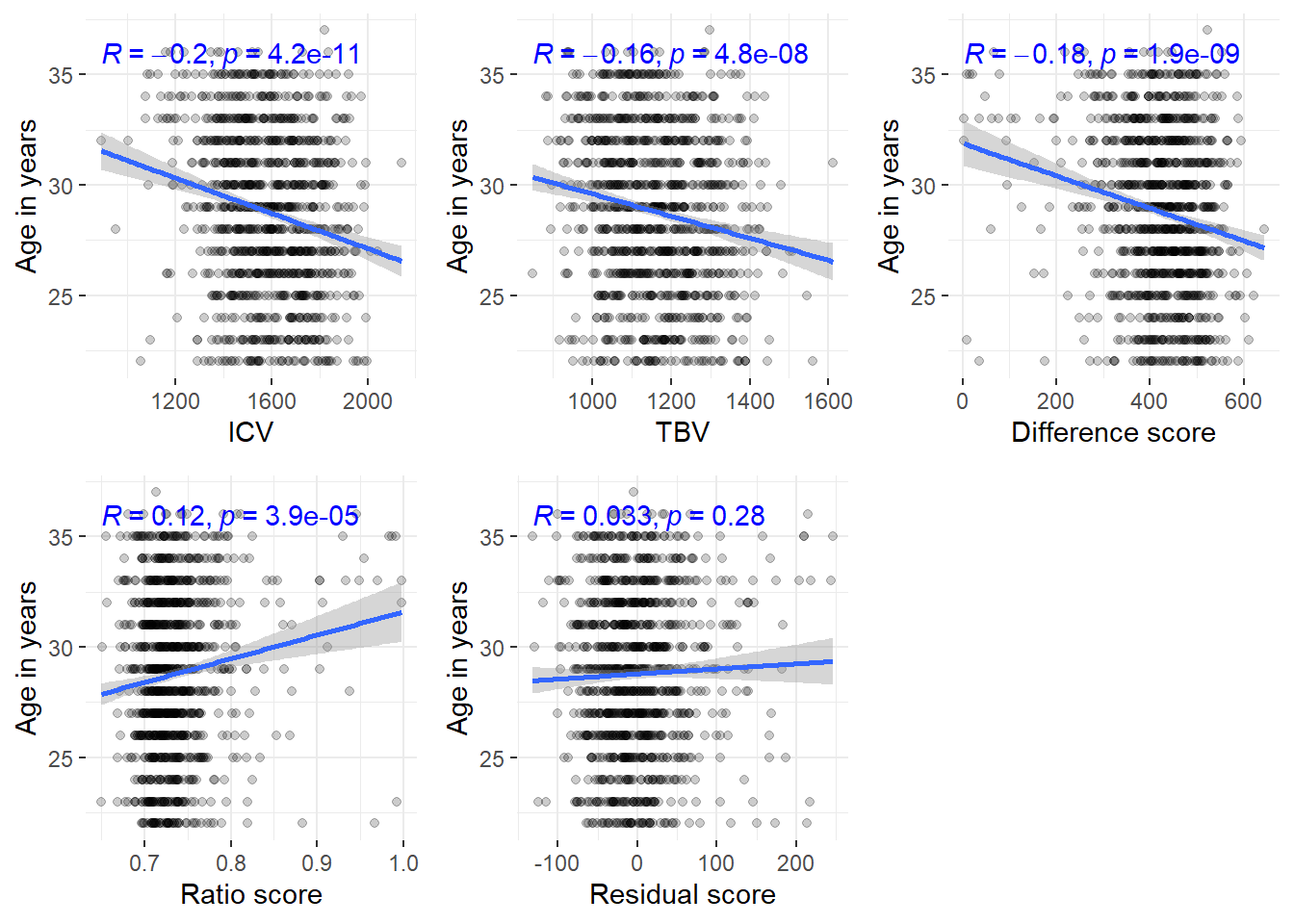

Excluding related individuals

• Relatedness is determined based on Family_ID variable

• The correlations stay about the same even when excluding all related individuals (N = 444)

Code

##### Family_ID
## Randomly select one participant from each family and keep  only one
HCPunrel = HCP[, .SD[sample(x = .N, size = 1)], by = Family_ID]

# calculate atrophy scores
HCPunrel$diff = HCPunrel$ICV - HCPunrel$TBV
HCPunrel$ratio = HCPunrel$TBV / HCPunrel$ICV

# delete those from data (none in this unrelated data)
if(sum(HCPunrel$diff < 0) != 0){HCPunrel=HCPunrel[-which(HCPunrel$diff < 0),]}

# estimate residual model
model <- lm(TBV ~ ICV, data = HCPunrel)
HCPunrel$resid = as.vector(resid(model, na.rm=T))

# standardise variables
HCPunrel$diff_stand = as.vector(scale(HCPunrel$diff))
HCPunrel$ratio_stand = as.vector(scale(HCPunrel$ratio))
HCPunrel$resid_stand = as.vector(scale(HCPunrel$resid))


########## plot age correlations (copied from Aim 1)
corICVunrel = ggplot(data = HCPunrel, aes(x = ICV, y = Age))+
  geom_point(alpha = 0.2)+
  theme_bw()+
  geom_smooth(method='lm')+
  stat_cor(method = "pearson",color ="blue")+
  ylab("Age in years")+
  theme(panel.border = element_blank())

corTBVunrel = ggplot(data = HCPunrel, aes(x = TBV, y = Age))+
  geom_point(alpha = 0.2)+
  theme_bw()+
  geom_smooth(method='lm')+
  stat_cor(method = "pearson",color ="blue")+
  ylab("Age in years")+
  theme(panel.border = element_blank())


cordiffunrel = ggplot(data = HCPunrel, aes(x = diff, y = Age))+
  geom_point(alpha = 0.2)+
  theme_bw()+
  geom_smooth(method='lm')+
  stat_cor(method = "pearson",color ="blue")+
  ylab("Age in years")+
  xlab("Difference score")+
  theme(panel.border = element_blank())

corratiounrel = ggplot(data = HCPunrel, aes(x = ratio, y = Age))+
  geom_point(alpha = 0.2)+
  theme_bw()+
  geom_smooth(method='lm')+
  stat_cor(method = "pearson",color ="blue")+
  ylab("Age in years")+
  xlab("Ratio score")+
  theme(panel.border = element_blank())

corresidunrel = ggplot(data = HCPunrel, aes(x = resid, y = Age))+
  geom_point(alpha = 0.2)+
  theme_bw()+
  geom_smooth(method='lm')+
  stat_cor(method = "pearson",color ="blue")+
  ylab("Age in years")+
  xlab("Residual score")+
  theme(panel.border = element_blank())

ggarrange(corICVunrel, corTBVunrel, cordiffunrel, corratiounrel, corresidunrel, common.legend=T, legend = "bottom")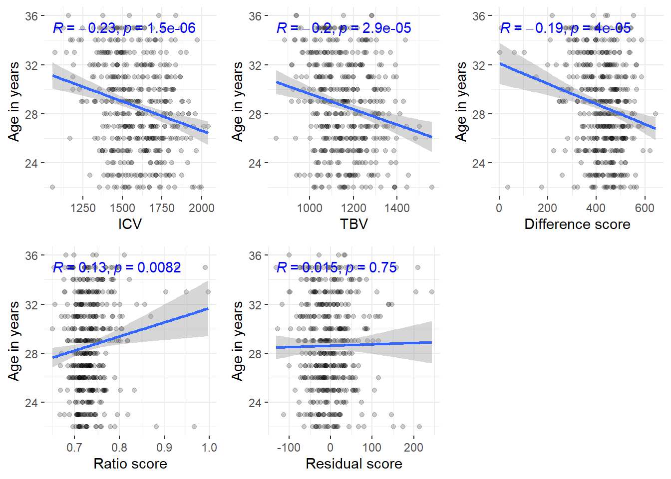

Adjusting for batch effects

Adjusting for batch effects does not change the strong age correlation we see in this young sample either.

Code

# adjust for Release and acquisition

# adjust ICV
model = lm('ICV ~ Release + Acquisition + fMRI_3T_ReconVrs', data =HCP)
summary(model)

Call:
lm(formula = "ICV ~ Release + Acquisition + fMRI_3T_ReconVrs", 
    data = HCP)

Residuals:
    Min      1Q  Median      3Q     Max 
-658.59 -118.49    0.97  129.22  550.84 

Coefficients:
                          Estimate Std. Error t value Pr(>|t|)    
(Intercept)               1519.335     93.893  16.182   <2e-16 ***
ReleaseQ1                  -40.029     75.514  -0.530    0.596    
ReleaseQ2                  -47.039     66.367  -0.709    0.479    
ReleaseQ3                  -47.600     59.833  -0.796    0.426    
ReleaseS1200                32.588     54.523   0.598    0.550    
ReleaseS500                 13.447     55.737   0.241    0.809    
ReleaseS900                -18.843     51.431  -0.366    0.714    
AcquisitionQ02              57.604     44.320   1.300    0.194    
AcquisitionQ03              45.814     59.384   0.771    0.441    
AcquisitionQ04              17.944     81.444   0.220    0.826    
AcquisitionQ05               5.692     83.162   0.068    0.945    
AcquisitionQ06               9.911     82.416   0.120    0.904    
AcquisitionQ07              43.858     80.984   0.542    0.588    
AcquisitionQ08              49.088     80.722   0.608    0.543    
AcquisitionQ09              57.448     81.066   0.709    0.479    
AcquisitionQ10              69.126     81.264   0.851    0.395    
AcquisitionQ11             102.821     81.136   1.267    0.205    
AcquisitionQ12              25.045     82.963   0.302    0.763    
AcquisitionQ13             -29.149     83.926  -0.347    0.728    
fMRI_3T_ReconVrsr177        37.644     61.707   0.610    0.542    
fMRI_3T_ReconVrsr177 r227   30.217     91.884   0.329    0.742    
fMRI_3T_ReconVrsr227        34.411     52.511   0.655    0.512    
---
Signif. codes:  0 '***' 0.001 '**' 0.01 '*' 0.05 '.' 0.1 ' ' 1

Residual standard error: 180.9 on 1081 degrees of freedom
Multiple R-squared:  0.03469,   Adjusted R-squared:  0.01594 
F-statistic:  1.85 on 21 and 1081 DF,  p-value: 0.01124

Code

HCP$ICVadj = resid(model)

corICV_adj = ggplot(data = HCP, aes(x = ICVadj, y = Age))+
  geom_point(alpha = 0.2)+
  theme_bw()+
  geom_smooth(method='lm')+
  stat_cor(method = "pearson",color ="blue")+
  ylab("Age in years")+
  xlab("ICV adjusted for Release and Acquisition")+
  theme(panel.border = element_blank())

# adjust TBV 
model = lm('TBV ~ Release + Acquisition', data =HCP)
HCP$TBVadj = resid(model)

corTBV_adj = ggplot(data = HCP, aes(x = TBVadj, y = Age))+
  geom_point(alpha = 0.2)+
  theme_bw()+
  geom_smooth(method='lm')+
  stat_cor(method = "pearson",color ="blue")+
  ylab("Age in years")+
  xlab("TBV adjusted for Release and Acquisition")+
  theme(panel.border = element_blank())

# re-create diff score with adjusted variables
HCP$diff_adj = HCP$ICVadj - HCP$TBVadj
  
cordiff_adj = ggplot(data = HCP, aes(x = diff_adj, y = Age))+
  geom_point(alpha = 0.2)+
  theme_bw()+
  geom_smooth(method='lm')+
  stat_cor(method = "pearson",color ="blue")+
  ylab("Age in years")+
  xlab("Difference score")+
  theme(panel.border = element_blank())

# re-create ratio score with adjusted variables
HCP$ratio_adj = HCP$TBVadj / HCP$ICVadj
 
corratio_adj = ggplot(data = HCP, aes(x = ratio_adj, y = Age))+
  geom_point(alpha = 0.2)+
  theme_bw()+
  geom_smooth(method='lm')+
  stat_cor(method = "pearson",color ="blue")+
  ylab("Age in years")+
  xlab("Ratio score")+
  theme(panel.border = element_blank())

ggarrange(corICV_adj, corTBV_adj, common.legend = T, legend = "bottom")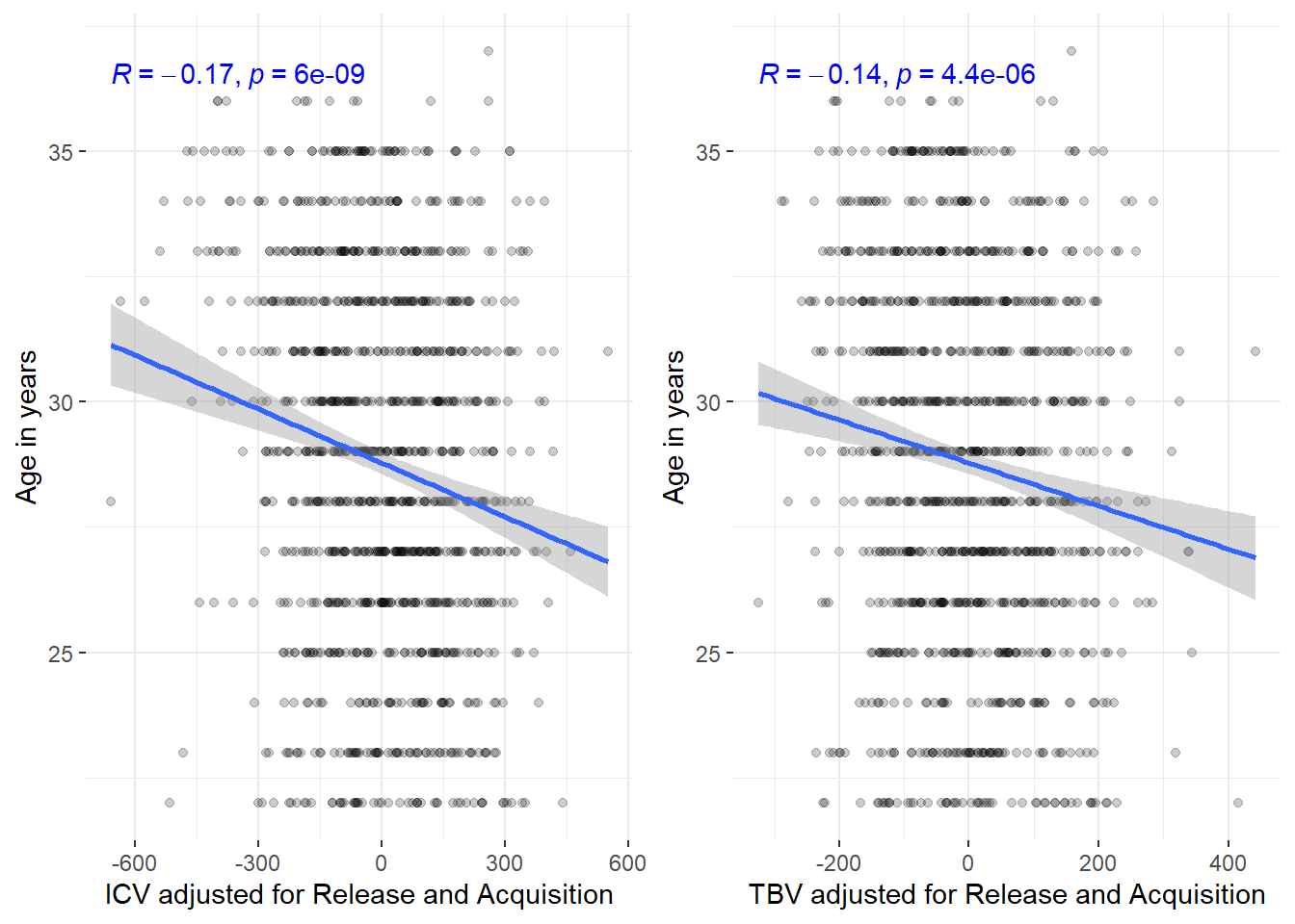

Restrict sample by age

• If we consider participants of and below 29 years only, the ICV age correlation disappears

• This threshold was empirically determined and then applied in the plot below

• In this younger sample, we see no age correlations whatsoever anymore

Determine most appropriate age cut-off for HCP

• the plot shows that the ICV-age correlation disappears at age 29 and below

• also this sample includes only 3 out of the 10 participants that had to get excluded due to ICV < TBV

Code

### determne which age is a good one to use for cut-off
# determine age cut-offs to iterate through
ageCut = seq(from = min(HCP$Age)+1, to = max(HCP$Age), by = 1)

# object to store results
storeNames = c("Age cut-off value", "Cor", "p", "ci_l", "ci_u", "Measure")
store = as.data.frame(matrix(nrow = length(ageCut), ncol = length(storeNames)))
names(store) = storeNames

# iterate over each age cut-off and calculate scores
for(i in ageCut){
  # store which age cut off iteration this is
  loc = which(is.na(store$`Age cut-off value`))[1]
  store[loc,"Age cut-off value"] = i
  
  # cut sample
  Youngdata = HCP[which(HCP$Age <= i),]
  
  # calculate correlations
  ## ICVerence
  store[loc,"Cor"] =
    with(Youngdata, cor.test(Age, ICV))$estimate
  
  store[loc,"p"] =
    with(Youngdata, cor.test(Age, ICV))$p.value
  
  store[loc,"ci_l"] =
    with(Youngdata, cor.test(Age, ICV))$conf.int[1]
  
  store[loc,"ci_u"] =
    with(Youngdata, cor.test(Age, ICV))$conf.int[2]
  
  store[loc,"Measure"] = "ICV"
}

ggplot(data = store)+
  geom_point(aes(x = Cor, y = `Age cut-off value`), alpha = 0.5)+
  geom_errorbar(aes(y = `Age cut-off value`, xmin = ci_l, xmax = ci_u), alpha = 0.3)+
  geom_vline(xintercept = -0.1, color = "grey")+
  geom_hline(yintercept = 31, color = "grey")+
  xlab("Correlation with age")+
  ylab("Age cut-off used to subset\nsample into a younger subsample")+
  scale_y_continuous(limits = c(21, 37.5), breaks = seq(from = 20, to = 36, by = 2))+
  ggtitle("Age-ICV correlation in HCP")+
  theme_bw()+
  theme(panel.border = element_blank())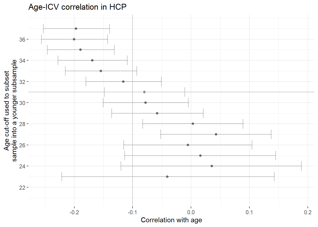

Explore age correlations in sample of or below 31 years

• When we restrict our sample to <= 31 years, the age correlations disappear

Code

HCPyoung = HCP[which(HCP$Age <= 31),]

# calculate atrophy scores
HCPyoung$diff = HCPyoung$ICV - HCPyoung$TBV
HCPyoung$ratio = HCPyoung$TBV / HCPyoung$ICV

# delete those from data 
#HCPyoung=HCPyoung[-which(HCPyoung$diff < 0),]

# estimate residual model
model <- lm(TBV ~ ICV, data = HCPyoung)
HCPyoung$resid = as.vector(resid(model, na.rm=T))


corICV = ggplot(data = HCPyoung, aes(x = ICV, y = Age))+
  geom_point(alpha = 0.2)+
  theme_bw()+
  geom_smooth(method='lm')+
  stat_cor(method = "pearson",color ="blue")+
  ylab("Age in years")+
  theme(panel.border = element_blank())

corTBV = ggplot(data = HCPyoung, aes(x = TBV, y = Age))+
  geom_point(alpha = 0.2)+
  theme_bw()+
  geom_smooth(method='lm')+
  stat_cor(method = "pearson",color ="blue")+
  ylab("Age in years")+
  theme(panel.border = element_blank())


cordiff = ggplot(data = HCPyoung, aes(x = diff, y = Age))+
  geom_point(alpha = 0.2)+
  theme_bw()+
  geom_smooth(method='lm')+
  stat_cor(method = "pearson",color ="blue")+
  ylab("Age in years")+
  xlab("Difference score")+
  theme(panel.border = element_blank())

corratio = ggplot(data = HCPyoung, aes(x = ratio, y = Age))+
  geom_point(alpha = 0.2)+
  theme_bw()+
  geom_smooth(method='lm')+
  stat_cor(method = "pearson",color ="blue")+
  ylab("Age in years")+
  xlab("Ratio score")+
  theme(panel.border = element_blank())

corresid = ggplot(data = HCPyoung, aes(x = resid, y = Age))+
  geom_point(alpha = 0.2)+
  theme_bw()+
  geom_smooth(method='lm')+
  stat_cor(method = "pearson",color ="blue")+
  ylab("Age in years")+
  xlab("Residual score")+
  theme(panel.border = element_blank())

ggarrange(corICV, corTBV, cordiff, corratio, corresid, common.legend=T, legend = "bottom")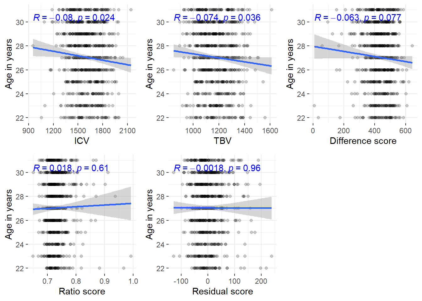

Plot distributions colored by age

Shown in Supplementary Figure 3: Distributions of TBV, ICV, and lifetime brain atrophy estimated with the residual, ratio, and difference method. Histograms are coloured by age groups.

Code

####################################################
# read in HCP data
HCP = fread(paste0(HCPdir,"/unrestricted_hcp_freesurfer.csv"))
HCP = HCP[,c("Subject", "Gender", "FS_InterCranial_Vol", "FS_BrainSeg_Vol_No_Vent")]
names(HCP) = c("ID", "Sex", "ICV", "TBV")

# add age information
HCPage = fread(paste0(HCPdir, "/RESTRICTED_annafurtjes_12_14_2023_4_18_2.csv"))
names(HCPage)[which(names(HCPage) == "Subject")] = "ID"
names(HCPage)[which(names(HCPage) == "Age_in_Yrs")] = "Age"
HCP = merge(HCP, HCPage[,c("ID","Age")], by = "ID")

# as outlined elsewhere, empirical investigations warrant to use an age cut-off of 31 years in this sample
HCP = HCP[which(HCP$Age <= 31),]

# convert mm3 estimates to more intuitive cm3 estimates
HCP$ICV = HCP$ICV/1000
HCP$TBV = HCP$TBV/1000

# estimate brain atrophy from single MRI scan
HCP$diff = HCP$ICV - HCP$TBV
HCP$ratio = HCP$TBV / HCP$ICV

# Quality control: 
#print(paste0("Some participants have negative difference scores and ratio scores > 1, which means that their ICV estimate is smaller than their TBV estimate. This must be an error as the skull always surrounds the brain. Those ", sum((HCP$diff < 0))," HCP participants were excluded from the data set."))

deletedHCP = sum(HCP$diff < 0)
# delete those from data 
if(sum(HCP$diff < 0) != 0){HCP=HCP[-which(HCP$diff < 0),]}

# estimate residual model
model <- lm(TBV ~ ICV, data = HCP)
HCP$resid = as.vector(resid(model, na.rm=T))

  
# standardise variables
HCP$diff_stand = as.vector(scale(HCP$diff))
HCP$ratio_stand = as.vector(scale(HCP$ratio))
HCP$resid_stand = as.vector(scale(HCP$resid))

####################################################
# make age groups
HCP$Age_group <- NA
HCP$Age_group[HCP$Age < 24] <- "23 years and under"
HCP$Age_group[HCP$Age >= 24 & HCP$Age < 25] <- "24"
HCP$Age_group[HCP$Age >= 25 & HCP$Age < 26] <- "25"
HCP$Age_group[HCP$Age >= 26 & HCP$Age < 27] <- "26"
HCP$Age_group[HCP$Age >= 27 & HCP$Age < 28] <- "27"
HCP$Age_group[HCP$Age >= 28 & HCP$Age < 29] <- "28"
HCP$Age_group[HCP$Age >= 29] <- "29 years and over"

p1=ggplot(HCP, aes(x=TBV, fill=Age_group)) +
  geom_histogram()+
  scale_fill_manual("Age groups", values = c("#292f56", "#1e4572", "#005c8b", "#008ba0", "#00bca1","#69e882", "#acfa70"))+
  xlab("TBV")+
  theme_bw()

p2=ggplot(HCP, aes(x=ICV, fill=Age_group)) +
  geom_histogram()+
  scale_fill_manual("Age groups", values = c("#292f56", "#1e4572", "#005c8b", "#008ba0", "#00bca1","#69e882", "#acfa70"))+
  xlab("ICV")+
  theme_bw()

p3=ggplot(HCP, aes(x=resid_stand, fill=Age_group)) +
  geom_histogram()+
  scale_fill_manual("Age groups", values = c("#292f56", "#1e4572", "#005c8b", "#008ba0", "#00bca1","#69e882", "#acfa70"))+
  xlab("Residual score")+
  theme_bw()

p4=ggplot(HCP, aes(x=ratio_stand, fill=Age_group)) +
  geom_histogram()+
  scale_fill_manual("Age groups", values = c("#292f56", "#1e4572", "#005c8b", "#008ba0", "#00bca1","#69e882", "#acfa70"))+
  xlab("Ratio score")+
  theme_bw()

p5=ggplot(HCP, aes(x=diff_stand, fill=Age_group)) +
  geom_histogram()+
  scale_fill_manual("Age groups", values = c("#292f56", "#1e4572", "#005c8b", "#008ba0", "#00bca1","#69e882", "#acfa70"))+
  xlab("Difference score")+
  theme_bw()

pHCP <- ggarrange(p1,p2,p3,p4,p5, nrow = 1, common.legend = T, legend = "bottom")
# add title
pHCP <- annotate_figure(pHCP, top = text_grob("HCP",face = "bold", size = 14))

#ggsave(paste0(out,"phenotypic/HCP_disttributions.jpg"), bg = "white",plot = pHCP, width = 30, height = 10, units = "cm", dpi = 300)
pHCP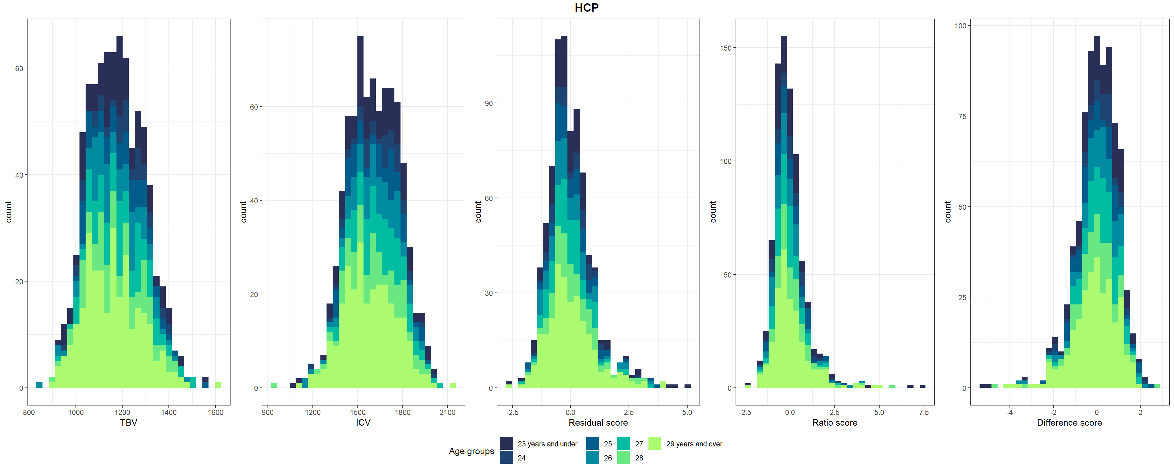

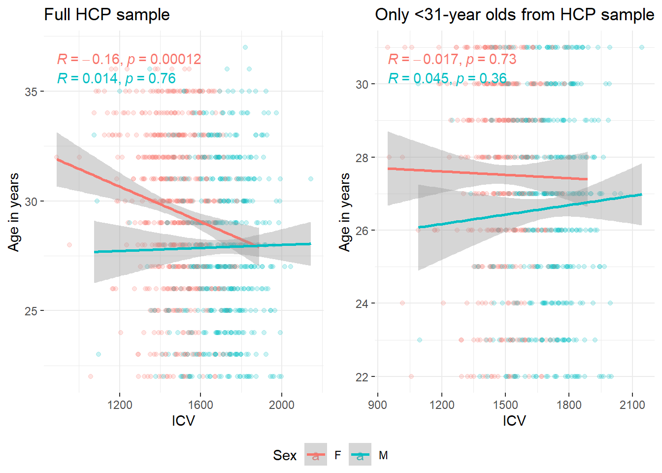
Sex effects

It was brought to our attention through the revision process of this project that the HCP has been shown to over-represent males at younger ages and that there are more females at older ages, which could also explain this effect here.

The plots below show a clear sex difference in ICV and TBV, as expected (i.e., larger ICV in males). It also shows that the unusual direction of effects (smaller heads at older ages) is driven by females.

Code

HCPcov = fread(paste0(HCPdir,list.files(path = HCPdir, pattern = "unrestricted_annafurtjes")))
HCPcov = HCPcov[,c("Subject", "Release", "Acquisition","fMRI_3T_ReconVrs")]

HCP = fread(paste0(HCPdir,"unrestricted_hcp_freesurfer.csv"))
HCP = HCP[,c("Subject", "Gender", "FS_InterCranial_Vol", "FS_BrainSeg_Vol_No_Vent")]

HCP = merge(HCP, HCPcov, by = "Subject")

HCPage = fread(paste0(HCPdir, "RESTRICTED_annafurtjes_12_14_2023_4_18_2.csv"))
HCPage = HCPage[,c("Subject","Age_in_Yrs", "Family_ID")]

HCP = merge(HCP, HCPage, by ="Subject")
names(HCP) = c("ID", "Sex", "ICV", "TBV", "Release", "Acquisition","fMRI_3T_ReconVrs", "Age", "Family_ID")

# convert mm3 estimates to more intuitive cm3 estimates
HCP$ICV = HCP$ICV/1000
HCP$TBV = HCP$TBV/1000

# calculate atrophy scores
HCP$diff = HCP$ICV - HCP$TBV
HCP$ratio = HCP$TBV / HCP$ICV

# delete those from data 
HCP=HCP[-which(HCP$diff < 0),]

# estimate residual model
model <- lm(TBV ~ ICV, data = HCP)
HCP$resid = as.vector(resid(model, na.rm=T))

# standardise variables
HCP$diff_stand = as.vector(scale(HCP$diff))
HCP$ratio_stand = as.vector(scale(HCP$ratio))
HCP$resid_stand = as.vector(scale(HCP$resid))

corICV = ggplot(data = HCP, aes(x = ICV, y = Age, color = Sex))+
  geom_point(alpha = 0.2)+
  stat_cor(aes(color = Sex), method = "pearson")+
  theme_bw()+
  geom_smooth(method='lm')+
  ylab("Age in years")+
  theme(panel.border = element_blank())+
  ggtitle("Full HCP sample")

corTBV = ggplot(data = HCP, aes(x = TBV, y = Age, color = Sex))+
  geom_point(alpha = 0.2)+
  stat_cor(aes(color = Sex), method = "pearson")+
  theme_bw()+
  geom_smooth(method='lm')+
  ylab("Age in years")+
  theme(panel.border = element_blank())

cordiff = ggplot(data = HCP, aes(x = diff, y = Age, color = Sex))+
  geom_point(alpha = 0.2)+
  theme_bw()+
  stat_cor(aes(color = Sex), method = "pearson")+
  geom_smooth(method='lm')+
  ylab("Age in years")+
  xlab("Difference score")+
  theme(panel.border = element_blank())

corratio = ggplot(data = HCP, aes(x = ratio, y = Age, color = Sex))+
  geom_point(alpha = 0.2)+
  theme_bw()+
  geom_smooth(method='lm')+
  ylab("Age in years")+
  xlab("Ratio score")+
  theme(panel.border = element_blank())

corresid = ggplot(data = HCP, aes(x = resid, y = Age, color = Sex))+
  geom_point(alpha = 0.2)+
  stat_cor(aes(color = Sex), method = "pearson")+
  theme_bw()+
  geom_smooth(method='lm')+
  ylab("Age in years")+
  xlab("Residual score")+
  theme(panel.border = element_blank())

ggarrange(corICV, corTBV, cordiff, corratio, corresid, common.legend=T, legend = "bottom")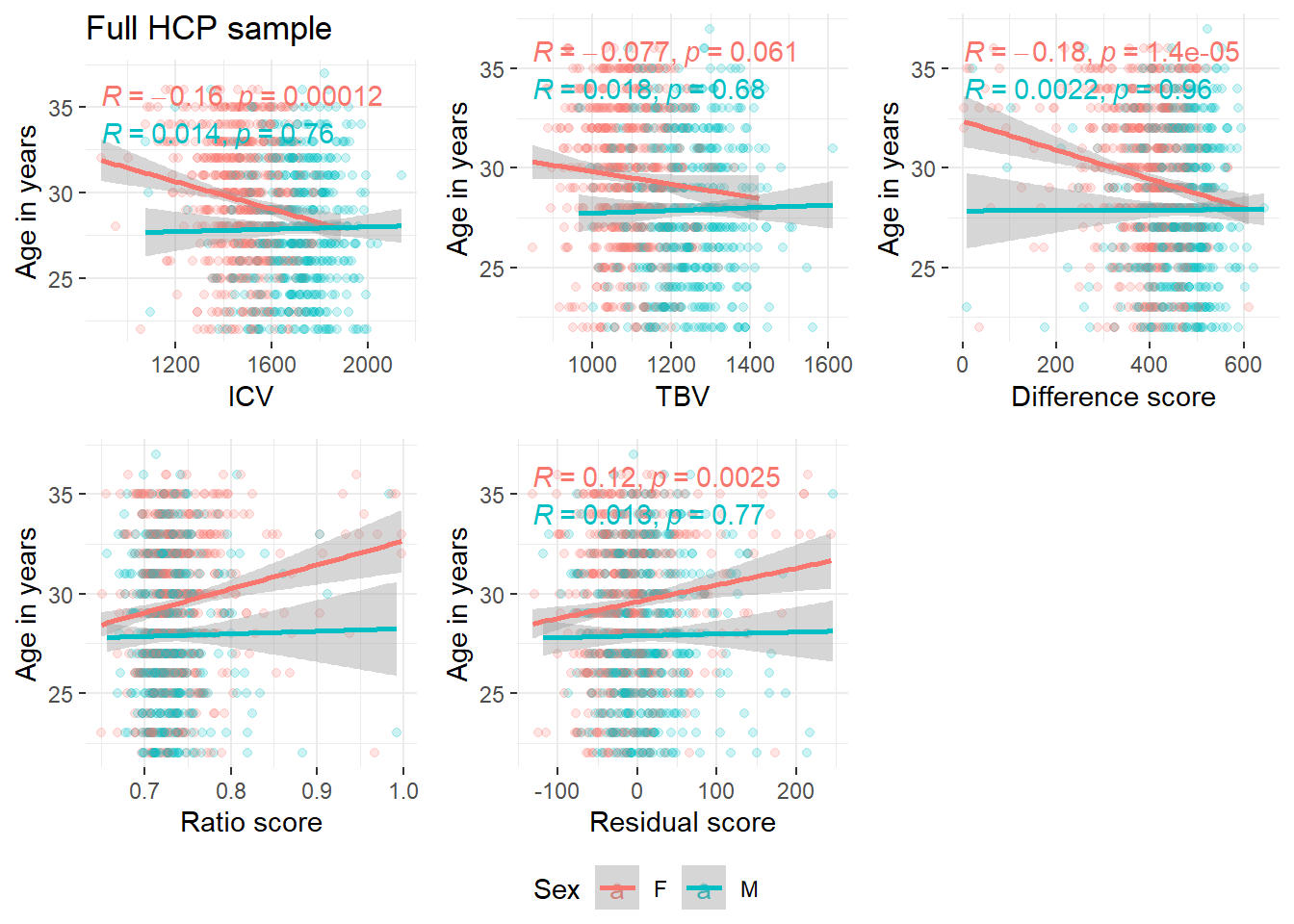

Code

####################################################
# read in HCP data
HCP = fread(paste0(HCPdir,"/unrestricted_hcp_freesurfer.csv"))
HCP = HCP[,c("Subject", "Gender", "FS_InterCranial_Vol", "FS_BrainSeg_Vol_No_Vent")]
names(HCP) = c("ID", "Sex", "ICV", "TBV")

# add age information
HCPage = fread(paste0(HCPdir, "/RESTRICTED_annafurtjes_12_14_2023_4_18_2.csv"))
names(HCPage)[which(names(HCPage) == "Subject")] = "ID"
names(HCPage)[which(names(HCPage) == "Age_in_Yrs")] = "Age"
HCP = merge(HCP, HCPage[,c("ID","Age")], by = "ID")

# convert mm3 estimates to more intuitive cm3 estimates
HCP$ICV = HCP$ICV/1000
HCP$TBV = HCP$TBV/1000

# estimate brain atrophy from single MRI scan
HCP$diff = HCP$ICV - HCP$TBV
HCP$ratio = HCP$TBV / HCP$ICV

# Quality control: 
#print(paste0("Some participants have negative difference scores and ratio scores > 1, which means that their ICV estimate is smaller than their TBV estimate. This must be an error as the skull always surrounds the brain. Those ", sum((HCP$diff < 0))," HCP participants were excluded from the data set."))

deletedHCP = sum(HCP$diff < 0)
# delete those from data 
if(sum(HCP$diff < 0) != 0){HCP=HCP[-which(HCP$diff < 0),]}

# estimate residual model for males and females separately
model <- lm(TBV ~ ICV, data = HCP)
HCP$resid = as.vector(resid(model, na.rm=T))

# estimate residual model for males and females separately
# males
#males <- HCP[HCP$Sex == "M",]
#model <- lm(TBV ~ ICV, data = males)
#males$resid = as.vector(resid(model, na.rm=T))

#females
#females <- HCP[HCP$Sex == "F",]
#model <- lm(TBV ~ ICV, data = females)
#females$resid = as.vector(resid(model, na.rm=T))

# merge males and females back together
#both = rbind(males,females)


# ICV
icv = ggplot(HCP, aes(y = ICV, x = Sex, fill = Sex))+
  geom_boxplot(alpha = 0.6, color = "black")+
  geom_point(aes(fill = factor(Sex)), 
             color = "grey45", 
             size = 2, 
             alpha = 0.5, 
             position = position_jitter(seed = 1, width = 0.2))+ 
  xlab("Sex")+
  ylab("ICV")+
  theme_bw()+
  theme(legend.position = "none")+
  theme(text = element_text(size=20),
        axis.text.x = element_text(size=20),#angle=45
        axis.text.y = element_text(size=20),
        axis.title.y = element_text(colour='black', size=20),
        axis.title.x = element_text(colour='black', size=20),
        plot.title = element_text(face = "bold", colour='black', size=20))

tbv = ggplot(HCP, aes(y = TBV, x = Sex, fill = Sex))+
  geom_boxplot(alpha = 0.6, color = "black")+
  geom_point(aes(fill = factor(Sex)), 
             color = "grey45", 
             size = 2, 
             alpha = 0.5, 
             position = position_jitter(seed = 1, width = 0.2))+ 
  xlab("Sex")+
  ylab("TBV")+
  theme_bw()+
  theme(legend.position = "none")+
  theme(text = element_text(size=20),
        axis.text.x = element_text(size=20),#angle=45
        axis.text.y = element_text(size=20),
        axis.title.y = element_text(colour='black', size=20),
        axis.title.x = element_text(colour='black', size=20),
        plot.title = element_text(face = "bold", colour='black', size=20))

# residual score
res = ggplot(HCP, aes(y = resid, x = Sex, fill = Sex))+
  geom_boxplot(alpha = 0.6, color = "black")+
  geom_point(aes(fill = factor(Sex)), 
             color = "grey45", 
             size = 2, 
             alpha = 0.5, 
             position = position_jitter(seed = 1, width = 0.2))+ 
  xlab("Sex")+
  ylab("Residual score (standardised)\n<- More brain atrophy      Less brain atrophy ->")+
  scale_fill_manual(values = c("#004225",  "#90ee90"))+
  theme_bw()+
  theme(legend.position = "none")+
  theme(text = element_text(size=20),
        axis.text.x = element_text(size=20),#angle=45
        axis.text.y = element_text(size=20),
        axis.title.y = element_text(colour='black', size=20),
        axis.title.x = element_text(colour='black', size=20),
        plot.title = element_text(face = "bold", colour='black', size=20))

# ratio score
rat = ggplot(HCP, aes(y = ratio, x = Sex, fill = Sex))+
  geom_boxplot(alpha = 0.6, color = "black")+
  geom_point(aes(fill = factor(Sex)), 
             color = "grey45", 
             size = 2, 
             alpha = 0.5, 
             position = position_jitter(seed = 1, width = 0.2))+ 
  xlab("Sex")+
  ylab("Ratio score (standardised)\n<- More brain atrophy      Less brain atrophy ->")+
  scale_fill_manual(values = c("#ffc40c",  "#fcffa4"))+
  theme_bw()+
  theme(legend.position = "none")+
  theme(text = element_text(size=20),
        axis.text.x = element_text(size=20),#angle=45
        axis.text.y = element_text(size=20),
        axis.title.y = element_text(colour='black', size=20),
        axis.title.x = element_text(colour='black', size=20),
        plot.title = element_text(face = "bold", colour='black', size=20))

# difference score
dif = ggplot(HCP, aes(y = diff, x = Sex, fill = Sex))+
  geom_boxplot(alpha = 0.6, color = "black")+
  geom_point(aes(fill = factor(Sex)), 
             color = "grey45", 
             size = 2, 
             alpha = 0.5, 
             position = position_jitter(seed = 1, width = 0.2))+ 
  xlab("Sex")+
  ylab("Ratio score (standardised)\n<- More brain atrophy      Less brain atrophy ->")+
  scale_fill_manual(values = c("#ff1493",  "#ffb6c1"))+
  theme_bw()+
  theme(legend.position = "none")+
  theme(text = element_text(size=20),
        axis.text.x = element_text(size=20),#angle=45
        axis.text.y = element_text(size=20),
        axis.title.y = element_text(colour='black', size=20),
        axis.title.x = element_text(colour='black', size=20),
        plot.title = element_text(face = "bold", colour='black', size=20))

plot_grid(icv, tbv, nrow = 1)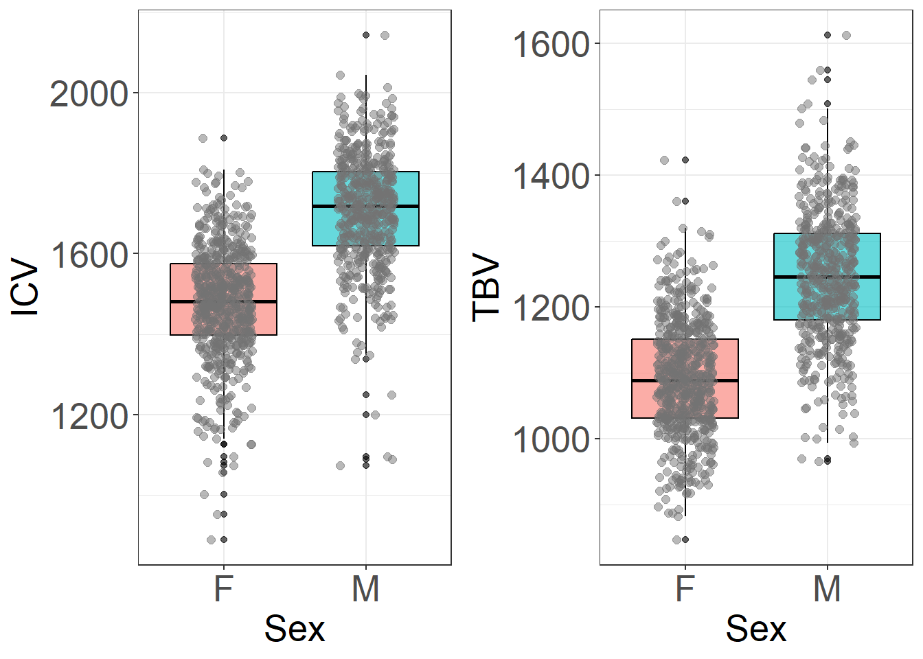

Test if sex effect is still there when restricting participants to <31 year-olds.

Code

# read in HCP data
HCP = fread(paste0(HCPdir,"/unrestricted_hcp_freesurfer.csv"))
HCP = HCP[,c("Subject", "Gender", "FS_InterCranial_Vol", "FS_BrainSeg_Vol_No_Vent")]
names(HCP) = c("ID", "Sex", "ICV", "TBV")

# add age information
HCPage = fread(paste0(HCPdir, "/RESTRICTED_annafurtjes_12_14_2023_4_18_2.csv"))
names(HCPage)[which(names(HCPage) == "Subject")] = "ID"
names(HCPage)[which(names(HCPage) == "Age_in_Yrs")] = "Age"
HCP = merge(HCP, HCPage[,c("ID","Age")], by = "ID")

# convert mm3 estimates to more intuitive cm3 estimates
HCP$ICV = HCP$ICV/1000

# as outlined elsewhere, empirical investigations warrant to use an age cut-off of 31 years in this sample
HCP = HCP[which(HCP$Age <= 31),]

#corICV 

corICV_below31= ggplot(data = HCP, aes(x = ICV, y = Age, color = Sex))+
  geom_point(alpha = 0.2)+
  stat_cor(aes(color = Sex), method = "pearson")+
  theme_bw()+
  geom_smooth(method='lm')+
  ylab("Age in years")+
  theme(panel.border = element_blank())+
  ggtitle("Only <31-year olds from HCP sample")

ggarrange(corICV, corICV_below31, common.legend = T, legend = "bottom")

`geom_smooth()` using formula = 'y ~ x'
`geom_smooth()` using formula = 'y ~ x'
`geom_smooth()` using formula = 'y ~ x'