Genome-wide association study

Author

Anna Elisabeth Furtjes

Published

June 6, 2025

Doi

10.1101/2024.11.06.622274

GWAS analysis was performed with the REGENIE software.

Input data was prepared using scripts for phenotypic and genotype data.

Ensure that the resid_stand variable was calculated in the subsample with non-missing data that is analysed in the GWAS analysis.

Regenie: Step 1

Code

#!/bin/bash

regenie_v3.4 \
--step 1 \
--bed $genotype/ukb_neuroimaging_brainAtrophy_GWASinput \
--phenoFile $phenotype/UKB_CrossNeuroIDP_noOutliers.txt \
--phenoColList ${trait}  \
--covarFile $phenotype/UKB_covarGWAS.txt \
--catCovarList sex,assessmentMonth,site,array,batch \
--bsize 100 \
--threads 30 \
--maxCatLevels 106 \
--lowmem \
--lowmem-prefix ${wd}/tmp_noOutliers \
--iid-only \
--out ${wd}/Step1_out_all_noOutliers

Regenie: Step 2

Code

#!/bin/bash

regenie_v3.4 \
--step 2 \
--bgen $imputed/ukb_chr${CHR}_clean_v3.bgen \
--sample $sampleFile/ukb10279_imp_chr${CHR}_v3_s487395.sample \
--keep $genotype/ukb_neuroimaging_brainAtrophy_GWASinput.fam \
--covarFile $phenotype/UKB_covarGWAS.txt \
--catCovarList sex,assessmentMonth,site,array,batch \
--maxCatLevels 106 \
--phenoFile $phenotype/UKB_CrossNeuroIDP_noOutliers.txt \
--phenoColList ${trait} \
--bsize 400 \
--minINFO 0.4 \
--minMAC 5 \
--threads 5 \
--pred ${step1}/Step1_out_all_pred_noOutliers.list \
--out $wd/GWAS_${trait}_chr${CHR}

Regenie interaction models: step 2

As unintuitive as it may seem, you must standardise the age variable before running this script. Regenie calculates a product-wise variable for the interaction between phenotype and age and if age is indicated in months or even days, the variable will be so large that regenie cannot handle it, and results will be massively inflated (results are complete nonsense with every SNP being extremely significant).

Code

#!/bin/bash

# note that this script only runs when linked to the bgen sample file 

trait=$1

for CHR in {1..22}
do
regenie_v3.4 \
--step 2 \
--bgen $imputed/ukb_chr${CHR}_clean_v3.bgen \
--ref-first \
--sample $sampleFile/ukb10279_imp_chr${CHR}_v3_s487395.sample \
--keep $genotype/ukb_neuroimaging_brainAtrophy_GWASinput.fam \
--covarFile $phenotype/UKB_covarGWAS.txt \
--catCovarList sex,assessmentMonth,site,array,batch \
--maxCatLevels 106 \
--phenoFile $phenotype/UKB_CrossNeuroIDP_noOutliers.txt \
--phenoColList ${trait} \
--bsize 400 \
--minINFO 0.4 \
--minMAC 5 \
--threads 5 \
--gz \
--interaction age \
--pred ${step1}/Step1_out_all_noOutliers_pred.list \
--out $wd/GWAS_${trait}_chr${CHR}_interaction
done

Format GWAS data

Code

library(data.table)
library(stringr)

# Read in the files for each area and merge them 
all_traits<-c("resid_stand","ratio_stand","diff_stand","TBVstand","ICVstand","CSFstand")

for(i in all_traits){

    # list all files that belong to this trait
    fileNames = list.files(pattern = i) 
    fileNames = fileNames[grepl(".regenie.gz", fileNames)]
    

    # exclude the 'interaction' GWAS
    fileNames = fileNames[!grepl("_interaction_", fileNames)]
    # include the 'interaction' GWAS
    #fileNames = fileNames[grepl("_interaction_", fileNames)]

    # sex split analyses
    #fileNames<-fileNames[grepl("_males", fileNames)]
    #i = paste0(i,"_males")

    # count number of chromosomes
    if(length(fileNames) != 22){warning(paste0(i, " GWAS has not got exactly 22 chromosome files!"))}

    # set object to count number of rows to 0
    count_rows<-0
    
    # object to hold GWAS
    dat <- data.frame()    

     for(j in fileNames){
            
       print(j)

        # read in file
       file<-fread(j,header=T,data.table=F)

        # if this is an interaction test, only keep interaction row for each SNP
        if(grepl("interaction", j)){
            
            # pull out the interaction effect from the full model
            file <- file[grepl("SNPxage", file$TEST),] 

            # if we're interested to look at attenuation of SNP effects, we can pull out ADD_INT_SNP which should represent the main effect of the tested SNP in the interaction model
            #file <- file[grepl("INT_SNP", file$TEST),] 
            # remove SNPxage
            #file <- file[!grepl("SNPxage", file$TEST),]
        }

        # merge
        dat <- rbind(dat, file) 
       
        # count number of rows 
        count_rows<-count_rows+nrow(file)
     }
    
    print("Done merging chromosome files")
    
    ## Sanity checks: Does the resulting file have the expected dimensions?
    if(nrow(dat)!= count_rows){print("Resulting merged file does not match the expected numeber of rows");break}
    
    if(ncol(dat) != 14){print("Resulting merged files does not match the expected number of columns"); break}
    
    print("File has dimensions as expected")
    print(dim(dat))
    
    # transform pvalues from log transformation to regular
    # https://www.biostars.org/p/358046/
    dat$P<-10^(-dat$LOG10P)
    #if(min(dat$P,na.rm=T)<=0 | max(dat$P,na.rm=T) >= 1){"Transformed p-value is out of bounds"; break}
    summary(dat$P)

    print("Done transform p-value column, and p-values are between 0 and 1")

    # create MAF column
    dat$MAF<-ifelse(dat$A1FREQ < 0.5, dat$A1FREQ, 1-dat$A1FREQ)

    # remove EXTRA column because it's empty
    dat$EXTRA <- NULL

    print(paste0("This is the file head for ",i))
    print(head(dat))
    
    # define file name to save the merged file
    fileName <- paste0("/finalGWAS/GWAS_brainAtrophy_", i,"_N43110.gz")
    
    # if this is an interaction run, name accordingly}               
    if(grepl("interaction", j)){
        #fileName <- paste0(wd,"/GWAS_brainAtrophy_", i,"_attenuatedMainEffects_N43110.gz")
        fileName <- paste0(wd,"/GWAS_brainAtrophy_", i,"_SNPxage_N43110.gz")
    }

    # save merged file
    fwrite(dat, fileName, na = "NA", quote = F, sep = "\t", row.names = FALSE, col.names = TRUE)
    
    print(paste0("Done writing file for ", i))
}

print("Done all traits")

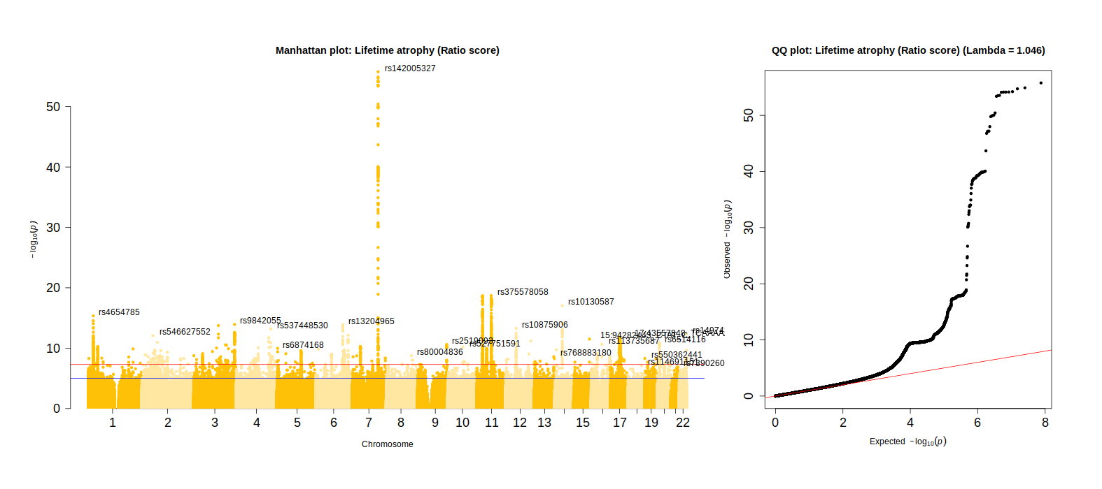
Manhattan plot

The scripts below were used to make Figure 4 in the main paper, and Supplementary Plots 15-19.

Alter Manhattan function for better looking annotation

This function was saved in a file called manhattan_big.R to be read in with source(manhattan_big.R) in the next step.

Code

manhattan_big <- function(x, chr="CHR", bp="BP", p="P", snp="SNP", 
                      col=c("gray10", "gray60"), chrlabs=NULL,
                      suggestiveline=-log10(1e-5), genomewideline=-log10(5e-8), 
                      highlight=NULL, logp=TRUE, annotatePval = NULL, annotateTop = TRUE, ...) {

    # Not sure why, but package check will warn without this.
    CHR=BP=P=index=NULL
    
    # Check for sensible dataset
    ## Make sure you have chr, bp and p columns.
    if (!(chr %in% names(x))) stop(paste("Column", chr, "not found!"))
    if (!(bp %in% names(x))) stop(paste("Column", bp, "not found!"))
    if (!(p %in% names(x))) stop(paste("Column", p, "not found!"))
    ## warn if you don't have a snp column
    if (!(snp %in% names(x))) warning(paste("No SNP column found. OK unless you're trying to highlight."))
    ## make sure chr, bp, and p columns are numeric.
    if (!is.numeric(x[[chr]])) stop(paste(chr, "column should be numeric. Do you have 'X', 'Y', 'MT', etc? If so change to numbers and try again."))
    if (!is.numeric(x[[bp]])) stop(paste(bp, "column should be numeric."))
    if (!is.numeric(x[[p]])) stop(paste(p, "column should be numeric."))
    
    # Create a new data.frame with columns called CHR, BP, and P.
    # d=data.frame(CHR=x[[chr]], BP=x[[bp]], P=x[[p]], pos = NA, index = NA) # with millions of SNPs, create dataframe at once 
                                                             #  rather than dynamically allocated(see line 72-73, and remove line 87 and line 91 )
    
    # If the input data frame has a SNP column, add it to the new data frame you're creating.
    if (!is.null(x[[snp]])) d = data.frame(CHR=x[[chr]], BP=x[[bp]], P=x[[p]], pos = NA, index = NA ,SNP=x[[snp]], stringsAsFactors = FALSE) else 
        d = data.frame(CHR=x[[chr]], BP=x[[bp]], P=x[[p]], pos = NA, index = NA)
        
    
    # Set positions, ticks, and labels for plotting
    ## Sort and keep only values where is numeric.
    #d <- subset(d[order(d$CHR, d$BP), ], (P>0 & P<=1 & is.numeric(P)))
    #  d <- subset(d, (is.numeric(CHR) & is.numeric(BP) & is.numeric(P)))       ## unused, all three variables are numeric, line:63-65 
    d <- d[order(d$CHR, d$BP), ]
    #d$logp <- ifelse(logp, yes=-log10(d$P), no=d$P)
    if (logp) {
        d$logp <- -log10(d$P)
    } else {
        d$logp <- d$P
    }
   # d$pos=NA
    
    
    # Fixes the bug where one chromosome is missing by adding a sequential index column.
   # d$index=NA
   # ind = 0
   # for (i in unique(d$CHR)){
   #     ind = ind + 1
   #     d[d$CHR==i,]$index = ind
   # }
   d$index = rep.int(seq_along(unique(d$CHR)), times = tapply(d$SNP,d$CHR,length))  # replcace the for loop of line 92-96 to improve efficiency
    
    # This section sets up positions and ticks. Ticks should be placed in the
    # middle of a chromosome. The a new pos column is added that keeps a running
    # sum of the positions of each successive chromsome. For example:
    # chr bp pos
    # 1   1  1
    # 1   2  2
    # 2   1  3
    # 2   2  4
    # 3   1  5
    nchr = length(unique(d$CHR))
    if (nchr==1) { ## For a single chromosome
        ## Uncomment the next two linex to plot single chr results in Mb
        #options(scipen=999)
        #d$pos=d$BP/1e6
        d$pos=d$BP
      #  ticks=floor(length(d$pos))/2+1          ## unused, from code line: 169
        xlabel = paste('Chromosome',unique(d$CHR),'position')
      #  labs = ticks          ## unused, from code line: 169
    } else { ## For multiple chromosomes
        lastbase=0
        ticks=NULL
        for (i in unique(d$index)) {
            if (i==1) {
                d[d$index==i, ]$pos=d[d$index==i, ]$BP
            } else {
        ## chromosome position maybe not start at 1, eg. 9999. So gaps may be produced. 
        lastbase = lastbase +max(d[d$index==(i-1),"BP"])   # replace line 128
        d[d$index == i,"BP"] = d[d$index == i,"BP"]-min(d[d$index==i,"BP"]) +1
        d[d$index == i, "pos"] = d[d$index == i,"BP"] + lastbase    # replace line 129
                # lastbase=lastbase+tail(subset(d,index==i-1)$BP, 1)
                # d[d$index==i, ]$pos=d[d$index==i, ]$BP+lastbase
           
            }
            # Old way: assumes SNPs evenly distributed
            # ticks=c(ticks, d[d$index==i, ]$pos[floor(length(d[d$index==i, ]$pos)/2)+1])
            # New way: doesn't make that assumption
           # ticks = c(ticks, (min(d[d$index == i,]$pos) + max(d[d$index == i,]$pos))/2 + 1)  # see line 136, to reduce the burden of for loop 
        }
    ticks <-tapply(d$pos,d$index,quantile,probs=0.5)   # replace line 135
        xlabel = 'Chromosome'
        #labs = append(unique(d$CHR),'') ## I forgot what this was here for... if seems to work, remove.
        labs <- unique(d$CHR)
    }
    
    # Initialize plot
    xmax = ceiling(max(d$pos) * 1.03)
    xmin = floor(max(d$pos) * -0.03)
    
    # The old way to initialize the plot
    # plot(NULL, xaxt='n', bty='n', xaxs='i', yaxs='i', xlim=c(xmin,xmax), ylim=c(ymin,ymax),
    #      xlab=xlabel, ylab=expression(-log[10](italic(p))), las=1, pch=20, ...)

    
    # The new way to initialize the plot.
    ## See http://stackoverflow.com/q/23922130/654296
    ## First, define your default arguments
    def_args <- list(xaxt='n', bty='n', xaxs='i', yaxs='i', las=1, pch=20,
                     xlim=c(xmin,xmax), ylim=c(0,ceiling(max(d$logp))),
                     xlab=xlabel, ylab=expression(-log[10](italic(p))))
    ## Next, get a list of ... arguments
    #dotargs <- as.list(match.call())[-1L]
    dotargs <- list(...)
    ## And call the plot function passing NA, your ... arguments, and the default
    ## arguments that were not defined in the ... arguments.
    do.call("plot", c(NA, dotargs, def_args[!names(def_args) %in% names(dotargs)]))
    
    # If manually specifying chromosome labels, ensure a character vector and number of labels matches number chrs.
    if (!is.null(chrlabs)) {
        if (is.character(chrlabs)) {
            if (length(chrlabs)==length(labs)) {
                labs <- chrlabs
            } else {
                warning("You're trying to specify chromosome labels but the number of labels != number of chromosomes.")
            }
        } else {
            warning("If you're trying to specify chromosome labels, chrlabs must be a character vector")
        }
    }
    
    # Add an axis. 
    if (nchr==1) { #If single chromosome, ticks and labels automatic.
        axis(1, ...)
    } else { # if multiple chrs, use the ticks and labels you created above.
        axis(1, at=ticks, labels=labs, ...)
    }
    
    # Create a vector of alternatiting colors
    #col=rep(col, max(d$CHR))  # replaced by line 187
    col = rep_len(col, max(d$index))  ## mean this one?  the results are same

    # Add points to the plot
    if (nchr==1) {
        with(d, points(pos, logp, pch=20, col=col[1], ...))
    } else {
        # if multiple chromosomes, need to alternate colors and increase the color index (icol) each chr.
        icol=1
        for (i in unique(d$index)) {
            #with(d[d$index==unique(d$index)[i], ], points(pos, logp, col=col[icol], pch=20, ...))
        points(d[d$index==i,"pos"], d[d$index==i,"logp"], col=col[icol], pch=20, ...)
            icol=icol+1
        }
    }
    
    # Add suggestive and genomewide lines
    if (suggestiveline) abline(h=suggestiveline, col="blue")
    if (genomewideline) abline(h=genomewideline, col="red")
    
    # Highlight snps from a character vector
    if (!is.null(highlight)) {
        if (any(!(highlight %in% d$SNP))) warning("You're trying to highlight SNPs that don't exist in your results.")
        d.highlight=d[which(d$SNP %in% highlight), ]
        with(d.highlight, points(pos, logp, col="green3", pch=20, ...)) 
    }
    
    # Highlight top SNPs
    if (!is.null(annotatePval)) {
        # extract top SNPs at given p-val
        if (logp) {
            topHits = subset(d, P <= annotatePval)
        } else
            topHits = subset(d, P >= annotatePval)
        par(xpd = TRUE)
        # annotate these SNPs
        if (annotateTop == FALSE) {
          if (logp) {
              with(subset(d, P <= annotatePval), 
                   textxy(pos, -log10(P), offset = 0.625, labs = topHits$SNP, cex = 1), ...)
          } else
              with(subset(d, P >= annotatePval), 
                   textxy(pos, P, offset = 0.625, labs = topHits$SNP, cex = 1), ...)
        }
        else {
            # could try alternative, annotate top SNP of each sig chr
            topHits <- topHits[order(topHits$P),]
            topSNPs <- NULL
            
            for (i in unique(topHits$CHR)) {
                
                chrSNPs <- topHits[topHits$CHR == i,]
                topSNPs <- rbind(topSNPs, chrSNPs[1,])
                
            }
            if (logp ){
                textxy(topSNPs$pos, -log10(topSNPs$P), offset = 0.625, labs = topSNPs$SNP, cex = 1, ...)
            } else
              textxy(topSNPs$pos, topSNPs$P, offset = 0.625, labs = topSNPs$SNP, cex = 1, ...)
        }
    }  
    par(xpd = FALSE)
}

Plot GWAS associations

Code

#######
# install.packages("R.utils") # to read .gz files
# install.packages("qqman")
# install.packages("calibrate")
library(data.table)
library(qqman)
library(calibrate)

# Manhattan plot

# loop through all traits
all_traits <- c("resid_stand", "ratio_stand", "diff_stand", "TBVstand", "ICVstand", "CSFstand")

for(trait_name in all_traits){

    dat = fread(list.files(pattern = paste0(trait_name, "_N")), data.table = F)

    ## remove MAF below 0.01
    dat = dat[dat$MAF > 0.01,]
    ## remove INFO below 0.8
    dat = dat[dat$INFO > 0.8,]

    ## for some reason the function plots too many SNP names below indicated threshold - reomve names 
    dat[which(dat$P > 5e-8), "ID"] = NA

    source(paste0(wd,"manhattan_big.R"))
    png(filename = paste0(wd, "/Manhattan",trait_name,"_clean.png"), width = 1575, height=700, units="px")

        layout_matrix <- matrix(1:2, nrow = 1, ncol=2)
        layout(layout_matrix,  widths = 2:1) #heights = 1.5:1,
        par(mar=c(5, 4, 4, 2))
        par(oma = c(3,3,3,3))

    # determine color for each of the comp methods
    if(trait_name == "resid_stand"){col = c("#004D40", "#00e7c0");pretty_name = "Lifetime atrophy (Residual score)"}
    if(trait_name == "ratio_stand"){col = c("#FFC107", "#FFE7a1"); pretty_name = "Lifetime atrophy (Ratio score)"}
    if(trait_name == "diff_stand"){col = c("#D81B60", "#F29ABA"); pretty_name = "Lifetime atrophy (Difference score)"}


    # Make MANHATTAN PLOT
    main = paste0("Manhattan plot: ", pretty_name)
    manhattan_big(dat, 
                main = main, 
                col = col, 
                chr="CHROM",
                bp="GENPOS",
                snp="ID",
                p="P", 
                annotatePval=-log10(5e-12),
                cex.axis = 1.5)

    # Assess systmeatic bias using Genomic Inflation factor
    # the genomic inflation factor is defined as the ratio of the median of the empirically observed distribution of test statistics to the expected mean, thus quantifying the extent of the bulk inflation and the excess false positive rate
    chisq <- qchisq(1-dat$P,1)
    lambda <- median(chisq)/qchisq(0.5,1)

    # make qq plot
    main <- paste0("QQ plot: ", pretty_name, " (Lambda = ", round(lambda, digits = 3), ")")
    qq(dat$P, main = main, cex = 1, cex.axis = 1.5)

    dev.off()
}

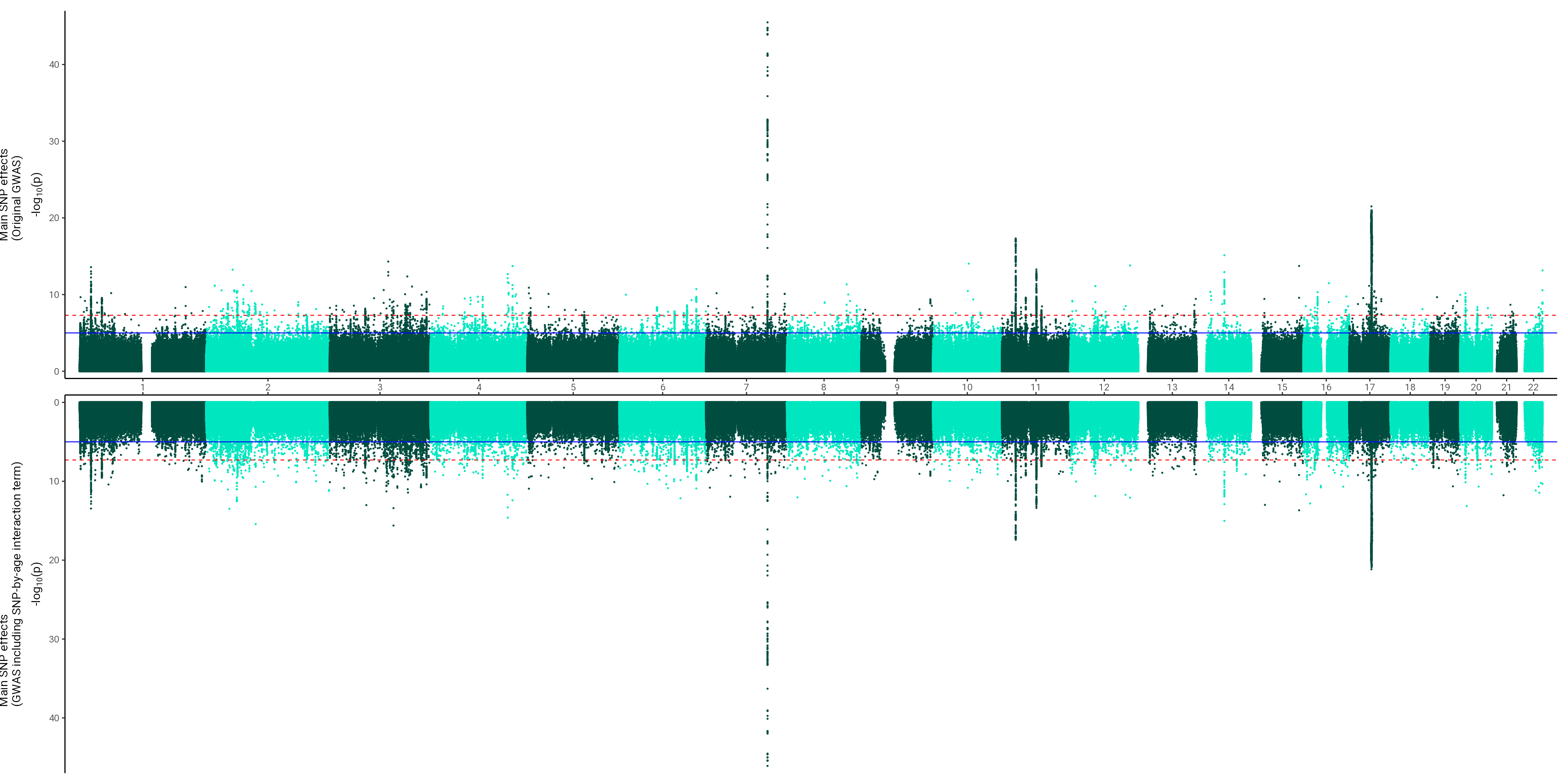
Miami plots

This script was used to generate Supplementary Plots 20-23 and 28-32.

Code

# Aim is to contrast main effects with the main effects that controlled for interaction effects for each of the three lifetime atrophy phenotypes

# 1. Read in main effects
# 2. Read in attenuated main effects
# 3. Create dummy columns to indicate which is which (will be used for split_by column)
# 4. Merge the two GWAS
# 5. Call function to contrast the two

library(data.table)
library(miamiplot)
library(ggplot2)

all_traits <- c("resid_stand", "ratio_stand", "diff_stand","TBVstand")

# set INFO filter
INFOfilter = 0.9

# keep only diallelic SNPs
diallelic = TRUE

# MAF filter
MAFfilter = 0.01

#i = all_traits[1]

for(i in all_traits){

    # 1. Read in main effects
    main = fread(list.files(pattern = paste0(i, "_N")), data.table = F)

    # dummy var
    main$split = 1

    # 2. Read in attenuated main effects
    #att = fread(list.files(pattern = paste0(i, "_attenuatedMainEffects")), data.table = F)
    att = fread(list.files(pattern = paste0(i, "_SNPxage")), data.table = F)
    # dummy var
    att$split = -1

    # some associations have a P value of 0 which will give an infinite value when transforming it into log
    # this is the case for 18,794 SNPs in resid GWAS for example, will exclude them here as plot otherwise does not work
    #att <- att[att$P != 0,]

    # 4. Merge the two GWAS
    merged = rbind(main, att)

    # if there is an info filter, filter for more reliable SNPs
    if(any(ls() == "INFOfilter")){merged <- merged[merged$INFO > INFOfilter,]}

    # if there is an MAF filter, filter for MAF
    if(any(ls() == "MAFfilter")){merged <- merged[merged$MAF > MAFfilter,]}

    # if diallelic has been set to TRUE, filter for diallelic SNPs only
    if(any(ls() == "diallelic")){   
        if(diallelic == T){
            merged <- merged[which(nchar(merged$ALLELE0) == 1),]
            merged <- merged[which(nchar(merged$ALLELE1) == 1),]
    }}

    #merged = merged[merged$CHROM == 1,] # for testing

    # summary(merged$P[which(merged$split == -1)])
    # summary(merged$P[which(merged$split == 1)])

    # clean up big files
    rm(list = c("att", "main"))

    # plot
    if(grepl("diff", i)){prettyName = "Difference score"; col = c("#D81B60", "#F29ABA")}
    if(grepl("ratio", i)){prettyName = "Ratio score"; col = c("#FFC107", "#FFE7a1")}
    if(grepl("resid", i)){prettyName = "Residual score"; col = c("#004D40", "#00e7c0")}
    if(grepl("TBV", i)){prettyName = "TBV"; col = c("#82A0D8","#8DDFCB")}

    ulabel = paste0("Main SNP effects\n(Original GWAS)")
    #llabel = paste0( "Main SNP effects\n(GWAS including SNP-by-age interaction term)")
    llabel = paste0( "SNP-by-age effects (Interaction GWAS)")

    p = ggmiami(data = merged, 
            chr = "CHROM",
            pos = "GENPOS",
            p = "P",
            split_by = "split", split_at = 0,
            upper_ylab = ulabel,
            lower_ylab = llabel,
            chr_colors = col)

    # save plot
    fileName = paste0(wd,"/miami_SNPxage_",i)

    # if INFO filter was used, write into file name
    if(any(ls() == "INFOfilter")){fileName = paste0(fileName,"_INFO", INFOfilter)}

    # if INFO filter was used, write into file name
    if(any(ls() == "MAFfilter")){fileName = paste0(fileName,"_MAF", MAFfilter)}

    # if only diallelic SNPs used, say in the name
    if(any(ls() == "diallelic")){
        if(diallelic == T){
            fileName = paste0(fileName, "_diallelic")
    }}

    fileName = paste0(fileName, "_2.png")

    ggsave(fileName, plot = p, width = 20, height = 10, dpi = 200)
}

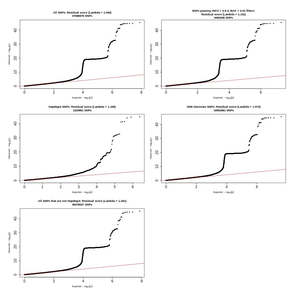
Examine QQ plots

This was used to generate Supplementary Plot 33.

Code

### examine why the qqplot seems so inflated
# plot qq all, MAF filter & INFO filter, hm3 SNPs (MAF > 0.01; INFO > 0.9), 1000G SNPs (MAF > 0.01; INFO > 0.9)

library(data.table)
library(qqman)
library(calibrate)
library(cowplot)
library(ggplot2)

# loop through all three traits
all_traits <- c("resid_stand", "ratio_stand", "diff_stand")

for(trait_name in all_traits){
    dat = fread(list.files(pattern = paste0(trait_name, "_N")), data.table = F)#, nrows = 200000
    #dat = dat[1:20000,]
    #dat = dat[dat$CHROM == 22,]

    # determine color for each of the comp methods
    if(trait_name == "resid_stand"){pretty_name = "Residual score"}
    if(trait_name == "ratio_stand"){pretty_name = "Ratio score"}
    if(trait_name == "diff_stand"){pretty_name = "Difference score"}

    # set up to save plot
    fileName <- paste0("/QQeval_",trait_name,".png")
    png(filename = fileName, width = 1000, height=1000, units="px")

        layout_matrix <- matrix(c(1,3,5,2,4,6), ncol=2, nrow=3)
        layout(layout_matrix,  widths = 1:1:1:1:1:1) #heights = 1.5:1,
        par(mar=c(5, 4, 4, 2))
        par(oma = c(3,3,3,3))


    ## PLOT 1: all SNPs
    ### Calculate Genomic Inflation factor
    chisq <- qchisq(1-dat$P,1)
    lambda <- median(chisq)/qchisq(0.5,1)

    # make qq plot
    main <- paste0("All SNPs: ", pretty_name, " (Lambda = ", round(lambda, digits = 3), ")\n", nrow(dat), " SNPs")
    p1 <- qq(dat$P, main = main, cex = 1, cex.axis = 1.5)

    ###############################
    ## PLOT 2: Apply INFO and MAF filter
    dat2 = dat[dat$MAF > 0.01,]
    dat2 = dat2[dat2$INFO > 0.8,]

    ### Calculate Genomic Inflation factor
    chisq <- qchisq(1-dat2$P,1)
    lambda <- median(chisq)/qchisq(0.5,1)

    # make qq plot
    main <- paste0("SNPs passing INFO > 0.9 & MAF > 0.01 filters:\n", pretty_name, " (Lambda = ", round(lambda, digits = 3), ")\n", nrow(dat2), " SNPs")
    p2 <- qq(dat2$P, main = main, cex = 1, cex.axis = 1.5)

    ###############################
    ## PLOT 3: HapMap3 SNPs only
    hm3 <- "eur_w_ld_chr/w_hm3.snplist"
    hm3SNPs <- fread(hm3)
    names(hm3SNPs) <- c("ID", "ALLELE1", "ALLELE0")

    # merge the two data sets and only keep overlapping SNPS that agree in A1 and A2
    dat2 <- merge(dat, hm3SNPs, by = "ID")

    ### Calculate Genomic Inflation factor
    chisq <- qchisq(1-dat2$P,1)
    lambda <- median(chisq)/qchisq(0.5,1)

    # make qq plot
    main <- paste0("HapMap3 SNPs: ", pretty_name, " (Lambda = ", round(lambda, digits = 3), ")\n", nrow(dat2), " SNPs")
    p3 <- qq(dat2$P, main = main, cex = 1, cex.axis = 1.5)
    
    ###############################
    ## PLOT 4: 1000 Genomes SNPs only
    # different reference files: this one is from FUMA website
    ref = "1KGphase3EURvariants.txt.gz"
    ref1000 <- fread(ref, select = c("SNP", "A1", "A2"))
    names(ref1000) <- c("ID", "ALLELE1", "ALLELE0")

    # merge the two data sets and only keep overlapping SNPS that agree in A1 and A2
    dat2 <- merge(dat, ref1000, by = "ID")

    ### Calculate Genomic Inflation factor
    chisq <- qchisq(1-dat2$P,1)
    lambda <- median(chisq)/qchisq(0.5,1)

    # make qq plot
    main <- paste0("1000 Genomes SNPs: ", pretty_name, " (Lambda = ", round(lambda, digits = 3), ")\n", nrow(dat2), " SNPs")
    p4 <- qq(dat2$P, main = main, cex = 1, cex.axis = 1.5)
    
    ###############################
    ## PLOT 5: HapMap3 SNPs removed
    # isolate SNPs not shared between data and hm3
    notHm3 = setdiff(dat$ID, hm3SNPs$ID)

    # only retain those 
    dat2 <- dat[dat$ID %in% notHm3,]
    
    ### Calculate Genomic Inflation factor
    chisq <- qchisq(1-dat2$P,1)
    lambda <- median(chisq)/qchisq(0.5,1)

    # make qq plot
    main <- paste0("All SNPs that are not HapMap3: ", pretty_name, " (Lambda = ", round(lambda, digits = 3), ")\n", nrow(dat2), " SNPs")
    p5 <- qq(dat2$P, main = main, cex = 1, cex.axis = 1.5)

    # save
    dev.off()
}