Descriptive statistics
\[\\[0.5in]\]
Here we calculate descriptive statistics for the brain networks.
\[\\[1in]\]
Phenotyic brain networks
Eigendecomposition
# set wd to where region names per network are saved
workingd<-getwd()
temporarywd<-paste0(workingd,"/Scripts/my_own_gwas/2Perform_ldsc")
setwd(temporarywd)

# load files containing region names
central_exec_regions<-read.table("central_executive_areas.txt")$V1
cingulo_regions<-read.table("cingulo_opercular_areas.txt")$V1
default_regions<-read.table("default_mode_areas.txt")$V1
hippocampal_regions<-read.table("hippocampal_diencephalic_areas.txt")$V1
multiple_demand_regions<-read.table("multiple_demand_areas.txt")$V1
p_fit_regions<-read.table("p_fit_areas.txt")$V1
salience_regions<-read.table("salience_areas.txt")$V1
sensori_regions<-read.table("sensorimotor_areas.txt")$V1
temporo_regions<-read.table("temporo_amygdala_orbitofrontal_areas.txt")$V1

# list the files
region_files<-ls(pattern="regions")

# create a dataframe to hold results
library(stringr)
descriptives_pheno_networks<-data.frame(networks=str_replace(region_files,pattern="_regions",replacement = ""))

# load phenotypic correlation matrix
temporarywd_pheno<-paste0(workingd,"/data_my_own/Pheno_preparation/")
setwd(temporarywd_pheno)

load("pheno_decomposition.RData")


for(i in region_files){
  #print(i)
  regions<-get(i)

  # get network specific matrix
  matrix<-cor_matrix[regions,regions]

  #calculate eigenvectors, eigenvalues and explained variances
  eigenvectors<-eigen(matrix)$vectors
  eigenvalues<-eigen(matrix)$values
  explained_variance<-round(eigenvalues/sum(eigenvalues)*100,digits = 3)
  #print(explained_variance)

  # save explained variance in object "descriptives_pheno_networks" in the appropriate row for each network
  network_name<-str_replace(i,pattern="_regions",replacement = "")
  descriptives_pheno_networks[which(descriptives_pheno_networks$networks == network_name),"R2"]<-explained_variance[1]

  # calculate standardised PC loadings
  stand_loadings<-eigenvectors%*%sqrt(diag(eigenvalues))
  stand_loadings<-stand_loadings[,1]

  # switch sign of stand loadings if median is negative
  if(sign(median(stand_loadings))==-1){
    stand_loadings<-stand_loadings*(-1)
  } else {
    stand_loadings<-stand_loadings
  }

  # save stand loadings for plot
  name_to_save<-paste0(network_name,"_pheno_loadings")
  assign(name_to_save,stand_loadings)

  # calculate mean,sd,median,min,max and save in object
  descriptives_pheno_networks[which(descriptives_pheno_networks$networks == network_name),"mean"]<-mean(stand_loadings)
  descriptives_pheno_networks[which(descriptives_pheno_networks$networks == network_name),"SD"]<-sd(stand_loadings)
  descriptives_pheno_networks[which(descriptives_pheno_networks$networks == network_name),"median"]<-median(stand_loadings)
  descriptives_pheno_networks[which(descriptives_pheno_networks$networks == network_name),"max"]<-max(stand_loadings)
  descriptives_pheno_networks[which(descriptives_pheno_networks$networks == network_name),"min"]<-min(stand_loadings)

  #calculate mode
    d<-density(stand_loadings)
    descriptives_pheno_networks[which(descriptives_pheno_networks$networks == network_name),"mode"]<-d$x[which.max(d$y)]
}

# add empty row to descriptives_pheno_networks
descriptives_pheno_networks[nrow(descriptives_pheno_networks)+1,]<-NA
descriptives_pheno_networks[which(is.na(descriptives_pheno_networks$networks)),"networks"]<-"whole_brain"

# eigendecomposition for the whole brain
eigenvectors<-eigen(cor_matrix)$vectors
eigenvalues<-eigen(cor_matrix)$values
explained_variance<-round(eigenvalues/sum(eigenvalues)*100,digits = 3)
descriptives_pheno_networks[which(descriptives_pheno_networks$networks == "whole_brain"),"R2"]<-explained_variance[1]

# calculate standardised PC loadings
  stand_loadings<-eigenvectors%*%sqrt(diag(eigenvalues))
  whole_brain_pheno_loadings<-stand_loadings[,1]*(-1)

# descriptive stats for the whole brain
  descriptives_pheno_networks[which(descriptives_pheno_networks$networks == "whole_brain"),"mean"]<-mean(whole_brain_pheno_loadings)
  descriptives_pheno_networks[which(descriptives_pheno_networks$networks == "whole_brain"),"SD"]<-sd(whole_brain_pheno_loadings)
  descriptives_pheno_networks[which(descriptives_pheno_networks$networks == "whole_brain"),"median"]<-median(whole_brain_pheno_loadings)
  descriptives_pheno_networks[which(descriptives_pheno_networks$networks == "whole_brain"),"max"]<-max(whole_brain_pheno_loadings)
  descriptives_pheno_networks[which(descriptives_pheno_networks$networks == "whole_brain"),"min"]<-min(whole_brain_pheno_loadings)

  #calculate mode
    d<-density(whole_brain_pheno_loadings)
    descriptives_pheno_networks[which(descriptives_pheno_networks$networks == "whole_brain"),"mode"]<-d$x[which.max(d$y)]

kable(descriptives_pheno_networks, digits = 2)| networks | R2 | mean | SD | median | max | min | mode |
|---|---|---|---|---|---|---|---|
| central_exec | 53.06 | 0.73 | 0.06 | 0.74 | 0.78 | 0.64 | 0.77 |
| cingulo | 38.69 | 0.60 | 0.17 | 0.70 | 0.78 | 0.33 | 0.72 |
| default | 36.49 | 0.59 | 0.13 | 0.61 | 0.76 | 0.40 | 0.67 |
| hippocampal | 38.09 | 0.61 | 0.10 | 0.58 | 0.76 | 0.50 | 0.54 |
| multiple_demand | 41.17 | 0.63 | 0.15 | 0.68 | 0.77 | 0.34 | 0.68 |
| p_fit | 34.12 | 0.57 | 0.12 | 0.57 | 0.74 | 0.30 | 0.56 |
| salience | 44.43 | 0.63 | 0.22 | 0.67 | 0.84 | 0.24 | 0.78 |
| sensori | 45.62 | 0.67 | 0.07 | 0.67 | 0.79 | 0.56 | 0.67 |
| temporo | 32.20 | 0.55 | 0.12 | 0.56 | 0.74 | 0.34 | 0.64 |
| whole_brain | 30.93 | 0.55 | 0.11 | 0.56 | 0.73 | 0.29 | 0.59 |
Plot density distribution of standardised loadings
data_pheno<-data.frame(matrix(ncol=2))
colnames(data_pheno)<-c("stand_loadings","network")

rm("regions_pheno_loadings")
loadings_pheno<-ls(pattern="pheno_loadings")
#names<-str_remove(loadings_pheno, pattern="_pheno_loadings")
#data_pheno$network<-names

for(i in loadings_pheno){
  df<-get(i)
  df<-unlist(df)
  #print(df)
  network<-str_remove(i, pattern="_pheno_loadings")
  #print(network)
  df<-cbind(df,network)
  colnames(df)<-c("stand_loadings","network")
  #print(df)
  #assign(i,df)
  data_pheno<-rbind(data_pheno,df)
}

# remove empty first row
data_pheno<-data_pheno[-1,]

# print full names for networks
data_pheno$network[which(data_pheno$network == "temporo")]<-"Temporo-amygdala-\norbitofrontal (30)"
data_pheno$network[which(data_pheno$network == "sensori")]<-"Sensorimotor (12)"
data_pheno$network[which(data_pheno$network == "salience")]<-"Salience (10)"
data_pheno$network[which(data_pheno$network == "p_fit")]<-"P-FIT (36)"
data_pheno$network[which(data_pheno$network == "multiple_demand")]<-"Multiple demand (12)"
data_pheno$network[which(data_pheno$network == "hippocampal")]<-"Hippocampal-\ndiencephalic (12)"
data_pheno$network[which(data_pheno$network == "default")]<-"Default mode (16)"
data_pheno$network[which(data_pheno$network == "cingulo")]<-"Cingulo-opercular (10)"
data_pheno$network[which(data_pheno$network == "central_exec")]<-"Central executive (8)"
data_pheno$network[which(data_pheno$network == "whole_brain")]<-"Whole brain (83 regions)"

# adjust data structure
data_pheno$network<-as.factor(data_pheno$network)
data_pheno$stand_loadings<-as.numeric(data_pheno$stand_loadings)

library(ggplot2)
library(RColorBrewer)
library(ggridges)

# Define the number of colors you want
nb.cols <- 10
mycolors <- colorRampPalette(brewer.pal(8, "Pastel1"))(nb.cols)

# save plot

#tiff("PC_pheno_loadings.tiff", width = 6.25, height = 5, units = 'in', res=1000)

 loadings_pheno_plot<-ggplot(data_pheno, aes(x=stand_loadings,y=network))+
              geom_density_ridges(rel_min_height = 0.005, aes(fill=as.factor(network)),stat="density_ridges", position = "identity", quantile_lines =TRUE,na.rm=TRUE, n=nrow(data_pheno)) +
              theme_ridges()+
              #scale_fill_brewer(values = mycolors)+
              scale_fill_manual(values=mycolors,guide=FALSE)+
              scale_x_continuous(n.breaks = 5)+
              xlab("Phenotypic PC loadings")+ylab("")+
              theme(legend.position = "none",
                    axis.text.x = element_text(size=26),
                    axis.text.y = element_text(size=26),
                    axis.title.x = element_text(face="bold",size=30),
                    panel.background = element_blank(),
                    axis.line = element_line(color="black"),
                    axis.line.x = element_line(color="black"))+theme_bw()
loadings_pheno_plot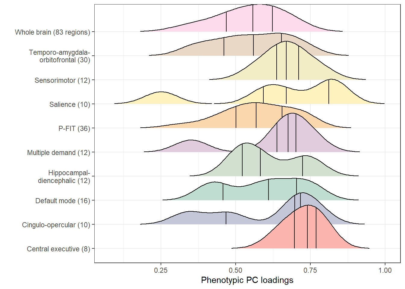
#dev.off()

# save network names and explained var in a new data.frame to plot further down
descriptives_pheno <- descriptives_pheno_networks[,c("networks","R2")]
names(descriptives_pheno)[which(names(descriptives_pheno) == "R2")] <- "pheno_R2"
Note that the vertical lines indicate quantiles.
Genetic brain networks
Eigendecomposition
### eigen decomposition of networks
rm(list=setdiff(ls(),c("loadings_pheno_plot","descriptives_pheno")))
library(stringr)
library(data.table)

# set wd where ldsc_output is saved
workingd<-getwd()
temporarywd<-paste0(workingd,"/data_my_own/ldsc/")
setwd(temporarywd)

# list available results in this directory
networks<-list.files(pattern=".RData")
network_names<-str_replace(networks,pattern=".RData",replacement = "")

# load results and name them after their corresponding network
for(i in 1:length(networks)){
  load(networks[i])
  name<-network_names[i]
    if(name == "whole_brain"){
      assign(name,LDSCoutput_wholebrain)
    }else{
      assign(name,LDSCoutput)
    }
}

# name rows and columns in matrices after their corresponding brain area
for(i in network_names){
  output<-get(i)
  dimnames(output$S_Stand)[[1]]<-dimnames(output$S)[[2]]
  dimnames(output$S_Stand)[[2]]<-dimnames(output$S)[[2]]
  name<-i
  assign(name,output)
  output$S_Stand<-round(output$S_Stand,digits = 2)
  name_cor<-paste0("cor_",i)
  assign(name_cor,output$S_Stand)
}

# list matrices of interest
matrices<-ls(pattern="cor_")

#create data frame with names of ldscoutput and names of correlation matrices
networks<-data.frame(cbind(matrices,network_names))

#######################################################
##### networks
#######################################################

for(i in 1:nrow(networks)){
    #### calculate eigenvectors
    # get correlation matrix of interest
    cormatrix<-get(matrices[i])

    # extract eigenvectors
    eigenvectors<-eigen(cormatrix)$vectors

    # get ldsc_output as it contains correct names (columns named after brain areas)
    noi<-get(network_names[i])

    # rename rows and columns with brain areas
    rownames(eigenvectors)<-dimnames(noi$S)[[2]]
    colnames(eigenvectors)<-dimnames(noi$S)[[2]]

    # save to network-specific variable name "eigenvectors"
    name<-paste0("eigenvectors_",network_names[i])
    assign(name,eigenvectors)

    ### calculate eigenvalues
    # extract eigenvalues
    eigenvalues<-eigen(cormatrix)$values

    # save to network-specific variable name "eigenvalues"
    name<-paste0("eigenvalues_",network_names[i])
    assign(name,eigenvalues)

    ### calculate explained_variances
    explained_variance<-round(eigenvalues/sum(eigenvalues)*100,digits = 3)
    name<-paste0("explained_var_",network_names[i])
    assign(name,explained_variance)

    ### calculate standardised loadings on first PC
    stand_loadings<-eigenvectors%*%sqrt(diag(eigenvalues))
    stand_loadings<-setDT(as.data.frame(stand_loadings), keep.rownames = TRUE)[,1:2]
    names(stand_loadings)<-c("Regions","stand_loadings")

    ### flip the loadings if median loadings are negative
    median_loadings<-median(stand_loadings$stand_loadings)
    mean_direction<-sign(median_loadings)
    if(mean_direction == -1){
    stand_loadings$stand_loadings<-stand_loadings$stand_loadings*(-1)
    } else {
    stand_loadings$stand_loadings<-stand_loadings$stand_loadings}

    name<-paste0("stand_loadings_",network_names[i])
    assign(name,stand_loadings)
    }

rm("stand_loadings")
loadings_all_traits<-ls(pattern="stand_loadings")

rm("explained_variance")
explained_all_traits<-ls(pattern="explained_var")
Save PC loadings in separate files
PC loadings are saved in a separate file to be able to create the network specific summary statistics in a later step, in which multiple regions are combined and weighted according to their PC loadings.
setwd(paste0(workingd,"/data_my_own/standardised_loadings/"))

for (i in loadings_all_traits){
    loadings<-get(i)
    file_name<-paste0(i,".txt")
    write.table(loadings,file=file_name,quote=F,sep=" ",na="NA",row.names=F,col.names = T)
}
# display the results in a table
library(knitr)
# create new dataframe with network names in one row
table<-data.frame(networks="test",matrix(nrow=10))[1]
table$networks<-str_replace(loadings_all_traits,pattern="stand_loadings_",replacement="")
for(i in 1:length(loadings_all_traits)){
# store explained var by first PC in every network
explained<-get(explained_all_traits[i])
table$explained[i]<-explained[1]
# calculate summary data and store in dataframe
loadings<-get(loadings_all_traits[i])
table$min[i]<-min(loadings$stand_loadings)
table$mean[i]<-mean(loadings$stand_loadings)
table$sd[i]<-sd(loadings$stand_loadings)
table$median[i]<-median(loadings$stand_loadings)
#calculate mode
d<-density(loadings$stand_loadings)
table$mode[i]<-d$x[which.max(d$y)]
table$max[i]<-max(loadings$stand_loadings)
}
table$number_included<-c(8,10,16,12,12,36,10,12,30,83)
kable(table,caption="Explained variance and loadings on first PC",format="markdown",digits=2,row.names = F)| networks | explained | min | mean | sd | median | mode | max | number_included |
|---|---|---|---|---|---|---|---|---|
| central_exec | 65.23 | 0.74 | 0.81 | 0.06 | 0.81 | 0.85 | 0.88 | 8 |
| cingulo | 47.50 | 0.52 | 0.68 | 0.12 | 0.67 | 0.66 | 0.90 | 10 |
| default_mode | 51.78 | 0.42 | 0.71 | 0.13 | 0.75 | 0.77 | 0.85 | 16 |
| hippocampal | 47.63 | 0.64 | 0.69 | 0.04 | 0.68 | 0.66 | 0.74 | 12 |
| multiple | 55.23 | 0.48 | 0.73 | 0.12 | 0.77 | 0.78 | 0.88 | 12 |
| p_fit | 47.56 | 0.43 | 0.68 | 0.09 | 0.69 | 0.69 | 0.83 | 36 |
| salience | 49.05 | 0.47 | 0.69 | 0.13 | 0.73 | 0.76 | 0.86 | 10 |
| sensori | 55.42 | 0.43 | 0.73 | 0.16 | 0.79 | 0.81 | 0.89 | 12 |
| temporo | 46.92 | 0.41 | 0.67 | 0.13 | 0.72 | 0.75 | 0.84 | 30 |
| whole_brain | 39.67 | 0.30 | 0.62 | 0.13 | 0.65 | 0.70 | 0.81 | 83 |
Plot density distribution of standardised loadings
# all networks are saved in loadings_all_traits

# add a column indicating network name to each df containing standardised loadings and volume names
# and save all in the same df called data_ridges
data_ridges<-data.frame(matrix(ncol=3))
colnames(data_ridges)<-c("Regions","stand_loadings","network")

for(i in loadings_all_traits){
  df<-get(i)
  name<-str_remove(i, pattern="stand_loadings_")
  df$network<-name
  #assign(i,df)
  data_ridges<-rbind(data_ridges,df)
}

# remove empty first row
data_ridges<-data_ridges[-1,]

# print full names for networks
data_ridges$network[which(data_ridges$network == "temporo")]<-"Temporo-amygdala-orbitofrontal"
data_ridges$network[which(data_ridges$network == "sensori")]<-"Sensorimotor"
data_ridges$network[which(data_ridges$network == "salience")]<-"Salience"
data_ridges$network[which(data_ridges$network == "p_fit")]<-"P-FIT"
data_ridges$network[which(data_ridges$network == "multiple")]<-"Multiple demand"
data_ridges$network[which(data_ridges$network == "hippocampal")]<-"Hippocampal-diencephalic"
data_ridges$network[which(data_ridges$network == "default_mode")]<-"Default mode"
data_ridges$network[which(data_ridges$network == "cingulo")]<-"Cingulo-opercular"
data_ridges$network[which(data_ridges$network == "central_exec")]<-"Central executive"
data_ridges$network[which(data_ridges$network == "whole_brain")]<-"Whole brain"


data_ridges$network<-as.factor(data_ridges$network)

library(ggplot2)
library(RColorBrewer)
library(ggridges)

# Define the number of colors you want
nb.cols <- 10
mycolors <- colorRampPalette(brewer.pal(8, "Pastel1"))(nb.cols)

# save plot

#tiff("PC_loadings.tiff", width = 6.25, height = 5, units = 'in', res=1000)

 loadings_plot<-ggplot(data_ridges, aes(x=stand_loadings,y=network))+
              geom_density_ridges(rel_min_height = 0.005, aes(fill=as.factor(network)),stat="density_ridges", position = "identity", quantile_lines =TRUE,na.rm=TRUE, n=nrow(data_ridges)) +
              theme_ridges()+
              #scale_fill_brewer(values = mycolors)+
              scale_fill_manual(values=mycolors,guide=FALSE)+
              scale_x_continuous(n.breaks = 5)+
              xlab("Genetic PC loadings")+ylab("")+
              theme(legend.position = "none",
                    axis.text.x = element_text(size=26),
                    axis.text.y = element_text(size=26),
                    axis.title.x = element_text(face="bold",size=30),
                    panel.background = element_blank(),
                    axis.line = element_line(color="black"),
                    axis.line.x = element_line(color="black"))+theme_bw()
loadings_plot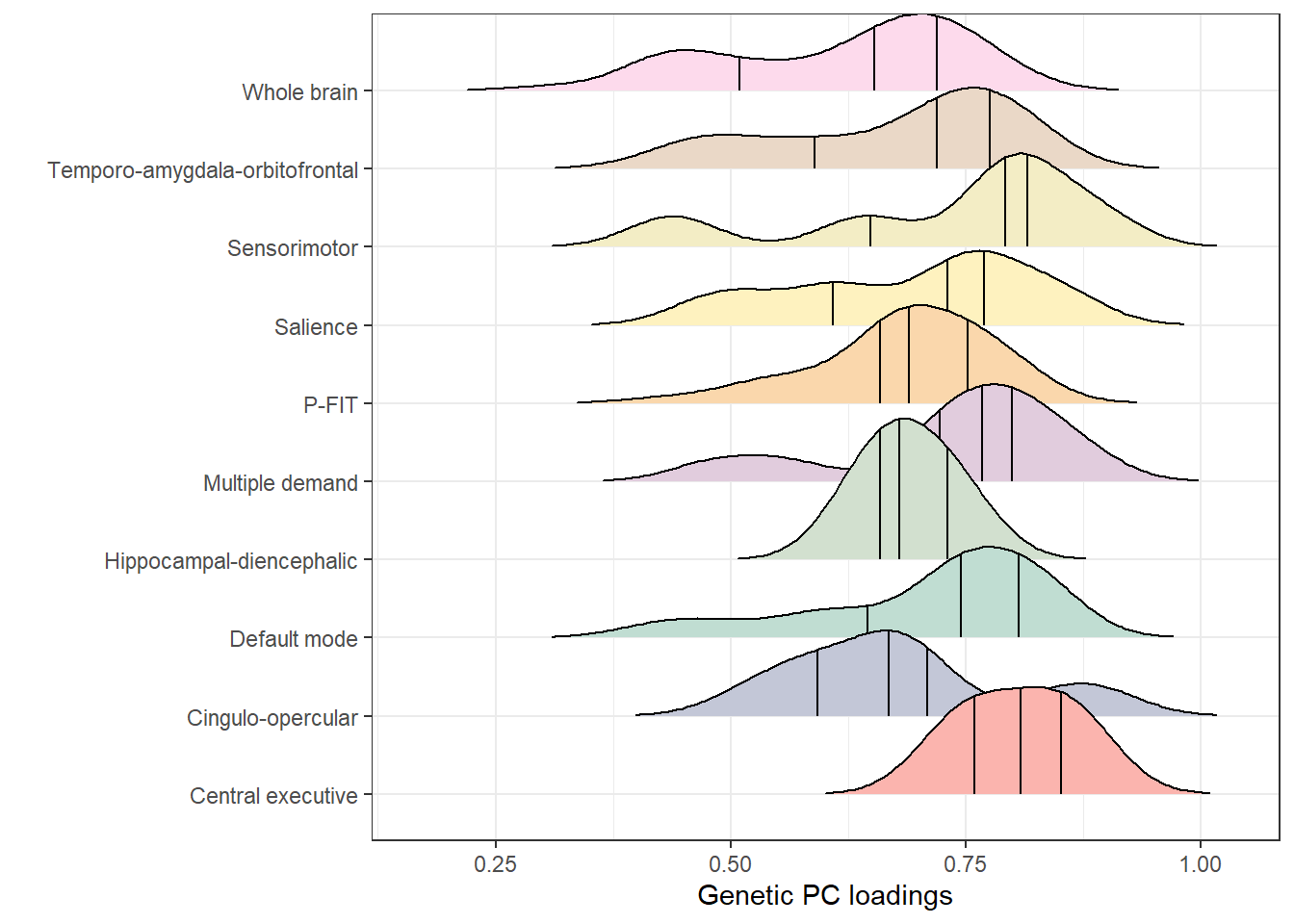
#dev.off()

# save without y axis to merge with phenotypic loadings in one figure below
loadings_plot <- loadings_plot + theme(axis.text.y = element_blank())
Note that the vertical lines indicate quantiles.
Plot explained variances
# save genetic descriptives to be plotted in a new data.frame
descriptives_geno <- table[,c("networks","explained")]
names(descriptives_geno)[which(names(descriptives_geno) == "explained")] <- "Genotype"

# rename networks so they match phenotypic names
descriptives_geno$networks[which(descriptives_geno$networks == "default_mode")]<-"default"
descriptives_geno$networks[which(descriptives_geno$networks == "multiple")]<-"multiple_demand"


# merge pheno and geno descriptive stats
descriptives <- merge(descriptives_pheno, descriptives_geno, by = "networks")
names(descriptives)[which(names(descriptives) == "pheno_R2")] <- "Phenotype"


# re-name the networks with how you want it to appear in the plot
descriptives$networks[which(descriptives$networks == "temporo")]<-"Temporo-amygdala-orbitofrontal"
descriptives$networks[which(descriptives$networks == "sensori")]<-"Sensorimotor"
descriptives$networks[which(descriptives$networks == "salience")]<-"Salience"
descriptives$networks[which(descriptives$networks == "p_fit")]<-"P-FIT"
descriptives$networks[which(descriptives$networks == "multiple_demand")]<-"Multiple demand"
descriptives$networks[which(descriptives$networks == "hippocampal")]<-"Hippocampal-diencephalic"
descriptives$networks[which(descriptives$networks == "default")]<-"Default mode"
descriptives$networks[which(descriptives$networks == "cingulo")]<-"Cingulo-opercular"
descriptives$networks[which(descriptives$networks == "central_exec")]<-"Central executive"
descriptives$networks[which(descriptives$networks == "whole_brain")]<-"Whole brain"

# round numbers for display
descriptives$Phenotype <- round(descriptives$Phenotype, digits = 1)
descriptives$Genotype <- round(descriptives$Genotype, digits = 1)

# melt data frame to plot
descriptives <- reshape2::melt(descriptives)
names(descriptives) <- c("networks","Modality","R2")

# choose  color
mycolors <- ifelse(descriptives$Modality == "Phenotype", "#ffd1dc","#77dd77")


# create vector for labels
library(dplyr)
labels <- descriptives %>% group_by(Modality) %>% summarise(
            label_x=R2,
            label_y=networks)

#labels <- descriptives

labels$label_position <- ifelse(labels$Modality == "Phenotype", labels$label_x-13, labels$label_x+13)


R2_plot <- ggplot(data=descriptives, aes(y=networks),shape=3)+
                            xlim(0,100)+
                            geom_point(aes(x=R2, fill = Modality), shape = 21, size=2, stroke = 1)+
                            labs(x = "% variance explained by 1st PC", y = "")+
                              theme_bw()+
                            geom_text(data = labels, aes(x=label_position, y=label_y, label=label_x), hjust = 0.5, vjust = 0.5, colour = "gray")


R2_plot
# save without y axis
R2_plot <- R2_plot + theme(axis.text.y = element_blank())
library(cowplot)
tiff("loadings_R2.tiff", width = 11, height = 6, units = 'in', res=1000)
plot_grid(loadings_pheno_plot,loadings_plot, R2_plot, nrow = 1,ncol = 3,labels=c("D","E","F"),width=1,height=1, label_size = 18,hjust = 0.07,scale = 0.85, rel_widths = c(1.5,1,1.5))
dev.off()
Parallel analysis for genetic networks
We test whether genetic PCs explain more variance than 95% of the corresponding PCs generated under a null model in a parallel analysis. We developed a version of parallel analysis to generate null distributions of eigenvalues by simulating null correlation matrices sampled from a diagonal population matrix, where the multivariate sampling distribution is specified to take the form of the sampling distribution of the standardized empirical genetic correlation matrix (V_Stand = sampling correlation matrix; S_Stand = genetic correlation matrix, as estimated using the ldsc function in GenomicSEM). This sampling correlation matrix (V_stand) serves as an index of the precision of and dependencies among genetic correlations when generating the random null data sets. We specify 1,000 replications to simulate the null correlation matrices and use a 95% threshold for distinguishing true eigenvalues from noise.
# load dependencies
library(stringr)

# load Javiers function
workingd<-getwd()
temporarywd<-paste0(workingd,"/Scripts/my_own_gwas/Eigendecomp/")
setwd(temporarywd)

source("Parallel_Anallysis_paLDSC_JF.R")

# load data and name it according to network
temporarywd<-paste0(workingd,"/data_my_own/ldsc/")
setwd(temporarywd)

networks<-list.files(pattern=".RData")
network_names<-str_replace(networks,pattern=".RData",replacement = "")

for(i in 1:length(networks)){
load(networks[i])
  name<-network_names[i]
  assign(name,LDSCoutput)
}

temporarywd<-paste0(workingd,"/data_my_own/PA_output/")
setwd(temporarywd)


for(i in network_names){
        ldsc_output<-get(i)
        paLDSC(S_Stand = ldsc_output$S_Stand, V_Stand = ldsc_output$V_Stand, r = 1000, p = .95, diag = F, fa = F, fm = "minres", save.pdf = T)
        name<-paste0("Parallel_analysis_",i,".pdf")
        file.rename("PCA_PA_LDSC.pdf",name)
}
Parallel analysis: Central Executive network

Parallel analysis: Cingulo-opercular network
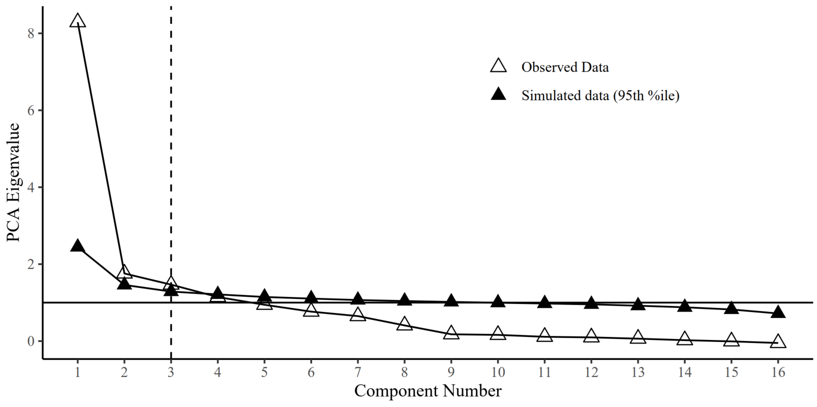
Parallel analysis: Default mode network
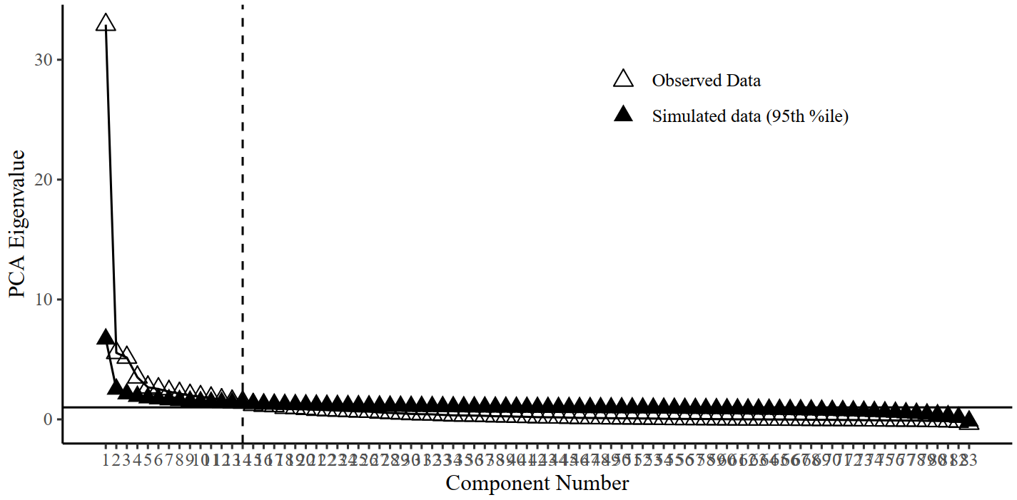
Parallel analysis: Whole-brain network (suggesting to extract 14 components)
Exploratory analyses
The first PC of larger networks explains less variance than the PC of smaller networks
volumes<-table$number_included
explained_var<-table$explained


cor.test(volumes,explained_var)
##
## Pearson's product-moment correlation
##
## data: volumes and explained_var
## t = -2.5803, df = 8, p-value = 0.0326
## alternative hypothesis: true correlation is not equal to 0
## 95 percent confidence interval:
## -0.9152174 -0.0770015
## sample estimates:
## cor
## -0.6739531plot(volumes,explained_var,ylab="Explained variance by first PC",xlab="Number of included volumes")
abline(lm(explained_var~volumes),col="red")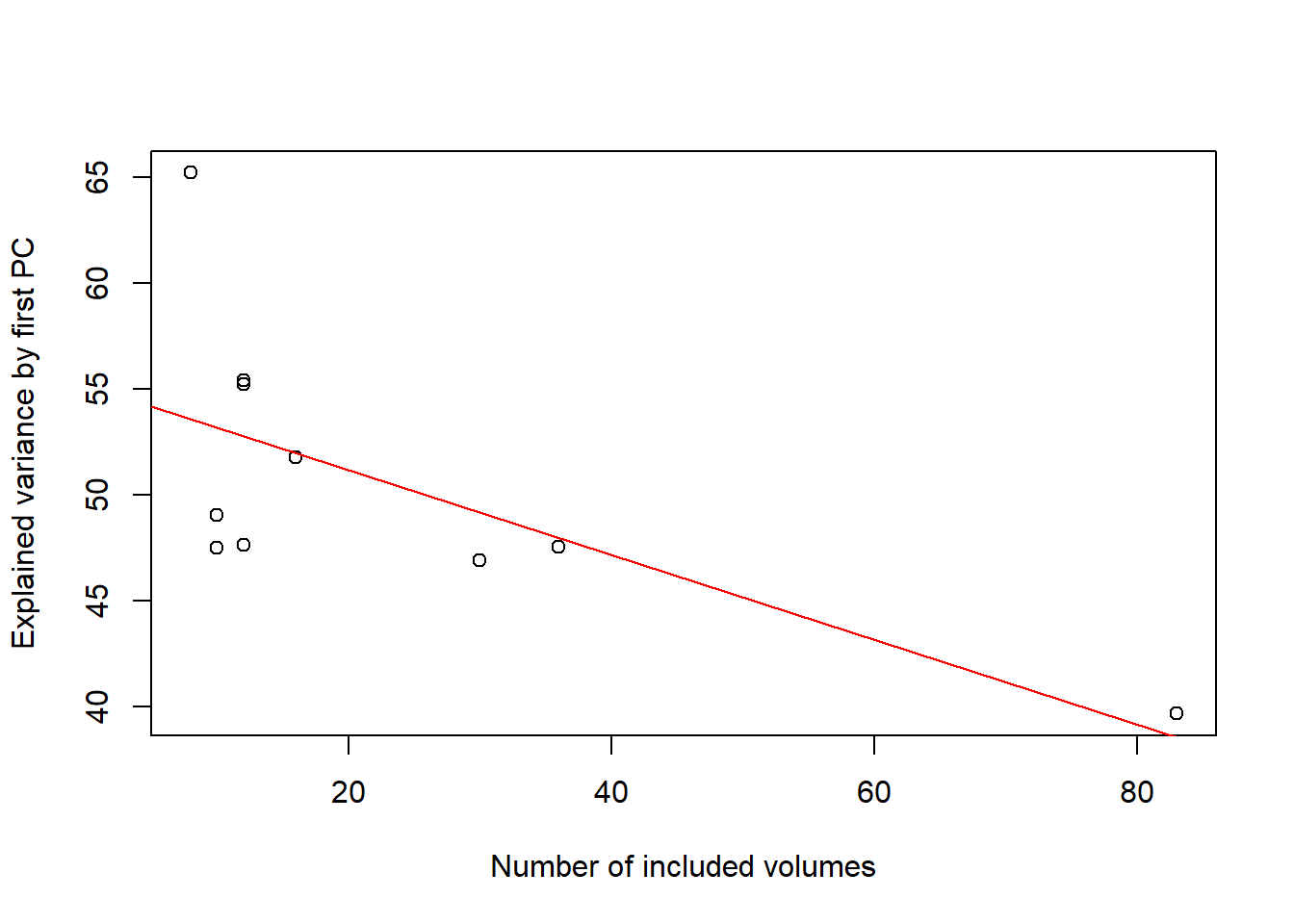
Parallel analysis suggests to extract more PCs for larger networks
networks<-c("central","cingulo","default","hippo","multiple","pfit","salience","sensori","temporo","whole_brain")
volumes<-table$number_included
components<-c(2,2,3,4,2,7,2,2,7,14)

test<-cbind(networks,volumes,components)

cor.test(volumes,components,data=test)
##
## Pearson's product-moment correlation
##
## data: volumes and components
## t = 14.313, df = 8, p-value = 5.54e-07
## alternative hypothesis: true correlation is not equal to 0
## 95 percent confidence interval:
## 0.9191324 0.9956563
## sample estimates:
## cor
## 0.981028plot(volumes,components,ylab="PCs with eigenvalues above chance",xlab="Number of included volumes")
abline(lm(components~volumes),col="red")
A priori networks explain more variance than networks with randomly included volumes
We added this analysis to formally test whether explained variances by the first underlying PC were larger for a priori networks than they were for networks including random volumes. The simulations are repeated for different amounts of randomly included volumes (800 times each), as the first PC of a network with fewer volumes generally explains less variance compared with networks including more volumes.
We ask this question, because it may invalidate a priori network characterisations if we obtain the same amounts of explained variances for random network characterisations.
# read in genetic correlation matrix - whole brain
workingd<-getwd()
temporarywd<-paste0(workingd,"/data_my_own/ldsc/")
setwd(temporarywd)

load("whole_brain.RData")
ldscoutput<-LDSCoutput_wholebrain

# name cells in genetic correlation matrix
dimnames(ldscoutput$S_Stand)[[1]]<-dimnames(ldscoutput$S)[[2]]
dimnames(ldscoutput$S_Stand)[[2]]<-dimnames(ldscoutput$S)[[2]]
ldscoutput$S_Stand<-ldscoutput$S_Stand

# randomly sample brain volumes to be included in a network
all_names<-dimnames(ldscoutput$S)[[2]]

# make table to save output
save_random<-data.frame(matrix(ncol=2))
colnames(save_random)<-c("number_included","random_R2")

# set seed for replicability
set.seed(1234)

# simulate for each number of included volumes in a priori networks
number_included<-c(8,10,12,16,30,36)

# set number of repititions per numver of included volumes
reps<-800

for(j in number_included){
    i<-0

      # repeat reps for each number of included volumes until reps is reached
      repeat{
        i<-i+1

        # determine row to be printed in
        row<-ifelse(nrow(save_random) == 0, 1,nrow(save_random)+1)

        # save number of volumes included
        save_random[row,"number_included"]<-j

        # randomly select volumes
        random_names<-sample(all_names, size=j)

        # eigendecomposition
        matrix<-ldscoutput$S_Stand[random_names,random_names]
        eigenvectors<-eigen(matrix)$vectors
        eigenvalues<-eigen(matrix)$values
        random_R2<-(eigenvalues/sum(eigenvalues)*100)[1]

        #save in table called save_random
        save_random[row,"random_R2"]<-random_R2

          if(i>=reps){
            break
          }
      }

}

# calculate statistics per number of included volumes

# mean
results_mean<-aggregate(save_random$random_R2, list(save_random$number_included), mean)
colnames(results_mean)<-c("number_included","random_R2_mean")

#sd
results_sd<-aggregate(save_random$random_R2, list(save_random$number_included), sd)
colnames(results_sd)<-c("number_included","random_R2_sd")
results<-merge(results_mean,results_sd,by="number_included")

#se
results_se<-cbind(number_included=results_sd$number_included, random_R2_se=results_sd$random_R2_sd/sqrt(reps))
results<-merge(results,results_se,by="number_included")

# confidence intervals
results$lower_ci<-with(results, random_R2_mean-(1.96*random_R2_se))
results$upper_ci<-with(results, random_R2_mean+(1.96*random_R2_se))

# round and merge confidence intervals for display
results$lower_ci<-round(results$lower_ci,digits = 2)
results$upper_ci<-round(results$upper_ci,digits = 2)

results$CI<-paste(results$lower_ci,results$upper_ci,sep=" - ")

# merge with empirical results
random_empirical<-merge(results[,c("number_included","random_R2_mean","CI")],table[,c("networks","explained","number_included")],by="number_included")

kable(random_empirical,digits = 2,caption="Mean explained variance and 95% confidence intervals for networks with randomly included volumes")| number_included | random_R2_mean | CI | networks | explained |
|---|---|---|---|---|
| 8 | 46.37 | 46.05 - 46.68 | central_exec | 65.23 |
| 10 | 45.01 | 44.72 - 45.31 | salience | 49.05 |
| 10 | 45.01 | 44.72 - 45.31 | cingulo | 47.50 |
| 12 | 43.99 | 43.72 - 44.25 | hippocampal | 47.63 |
| 12 | 43.99 | 43.72 - 44.25 | multiple | 55.23 |
| 12 | 43.99 | 43.72 - 44.25 | sensori | 55.42 |
| 16 | 42.61 | 42.38 - 42.83 | default_mode | 51.78 |
| 30 | 40.86 | 40.72 - 41.01 | temporo | 46.92 |
| 36 | 40.59 | 40.45 - 40.72 | p_fit | 47.56 |
All nine a priori networks explain more variance than networks with randomly selected volumes. Comparisons must be made for matching numbers of included volumes (i.e. the 39% explained variance by the central executive network should be compared with the mean explained variance for networks with 8 randomly selected regional volumes).
Plot PC1 loadings
rm(list=ls())
library(ggseg)
library(dplyr)
library(ggpubr)
#####################################################################################
### Read in data
#####################################################################################

# load data and name it according to network
workingwd<-getwd()
temporarywd<-paste0(workingwd,"/data_my_own/standardised_loadings/")
setwd(temporarywd)

networks<-list.files(pattern=".txt")
network_names<-str_replace(networks,pattern=".txt",replacement = "")
network_names<-str_replace(network_names,pattern="stand_loadings_",replacement = "")

# save region names that ggseg understands/ frame dk will be available as soon as ggseg library was loaded
Regions = as.data.frame(cbind(dk$data$region, dk$data$hemi))
names(Regions)=c("region","hemi")
# remove NAs
Regions <- Regions[-which(is.na(Regions$region)),]

# save subcortical region names that ggseg understands
Regions_sub <- as.data.frame(aseg$data[,c("hemi","region","side")])
# remove missing names
Regions_sub <- Regions_sub[which(!is.na(Regions_sub$region)),]

# make object to store plots
plots <- list()

# read in standardised loadings & rename according to ggseg convention
for(i in 1:length(networks)){
  # read in standardised loadings
  load <- read.table(networks[i], header = TRUE)

  ### harmonise names to match ggseg naming
  names(load)[which(names(load) == "Regions")] <- "region"
  # determine hemi
  load$hemi <- "right"
  load$hemi[grep("Left_", load$region)] <- "left"


  # adjust region names to match ggseg naming
  # remove "Left_" from region name
  load$region = str_remove(pattern = "Left_", load$region)
  # remove "Right_" from region name
  load$region = str_remove(pattern = "Right_", load$region)
  # replace _ with space
  load$region = str_replace_all(load$region, pattern="_", replacement = " ")

  # remove subcortical regions
  load_cort = load[load$region %in% Regions$region,]


  # plot PC loadings and save
  plot_cortical <-
    load_cort %>%
    ggplot() +
    geom_brain(atlas = dk,
               position = position_brain(hemi ~ side),
               aes(fill = stand_loadings)) +
    labs(fill = "PC1\nloadings")+
    theme_bw()+
    scale_fill_continuous(limits = c(0, 1), type = "viridis")+
    #scale_color_gradient(low = "red", high = "blue")+
    theme(text = element_text(size=15),
          axis.text.x = element_blank(),
          axis.text.y = element_blank(),
          axis.title.y = element_text(face="bold", colour='#1A1A1A', size=20),
          axis.title.x = element_blank(),
          axis.line.x = element_blank(),
          axis.line.y = element_blank(),
          axis.ticks.x = element_blank(),
          axis.ticks.y = element_blank(),
          panel.border = element_blank())

  # add title
  if(network_names[i] == "central_exec"){
      name <- "Central executive"
  }else if(network_names[i] == "cingulo"){
      name <- "Cingulo-opercular"
  }else if(network_names[i] == "default_mode"){
      name <- "Default mode"
  }else if(network_names[i] == "hippocampal"){
      name <- "Hippocampal"
  }else if(network_names[i] == "multiple"){
      name <- "Multiple demand"
  }else if(network_names[i] == "p_fit"){
      name <- "P-FIT"
  }else if(network_names[i] == "salience"){
      name <- "Salience"
  }else if(network_names[i] == "sensori"){
      name <- "Sensorimotor"
  }else if(network_names[i] == "temporo"){
      name <- "Temporo-amygdala-\norbitofrontal"
  }else if(network_names[i] == "whole_brain"){
      name <- "Whole brain"
  }

  plot_cortical <- plot_cortical + ggtitle(name)

  # pick name
  name2<-network_names[i]

  # store plot
  plots[[name2]]<-plot_cortical


  ##### plot subcortical
  # brain stem has capital letter
  load$region <- tolower(load$region)
  # keep subcortcal regions only
  load_sub <-  load[load$region %in% Regions_sub$region,]

  # only plot if there are subcortical regions
  if(nrow(load_sub) != 0){


      # add side as in ggseg
      load_sub$side <- "coronal"
      load_sub$side <- ifelse(load_sub$region == "brain stem", "sagittal", "coronal")
      # brain stem is on midline
      load_sub$hemi[which(load_sub$region == "brain stem")] <- "midline"

      plot_sub <-
          load_sub %>%
          ggplot() +
          geom_brain(atlas = aseg,
                     aes(fill = stand_loadings)) +
          labs(fill = "PC1\nloadings")+
          theme_bw()+
          scale_fill_continuous(limits = c(0, 1), type = "viridis")+
          theme(text = element_text(size=15),
                axis.text.x = element_blank(),
                axis.text.y = element_blank(),
                axis.title.y = element_text(face="bold", colour='#1A1A1A', size=20),
                axis.title.x = element_blank(),
                axis.line.x = element_blank(),
                axis.line.y = element_blank(),
                axis.ticks.x = element_blank(),
                axis.ticks.y = element_blank(),
                panel.border = element_blank())+
        ggtitle(name)

      # pick name
      name<-paste0("sub_",network_names[i])
      # store plot
      plots[[name]]<-plot_sub

  }
}

ggarrange(plotlist = plots, common.legend = TRUE, legend = "right")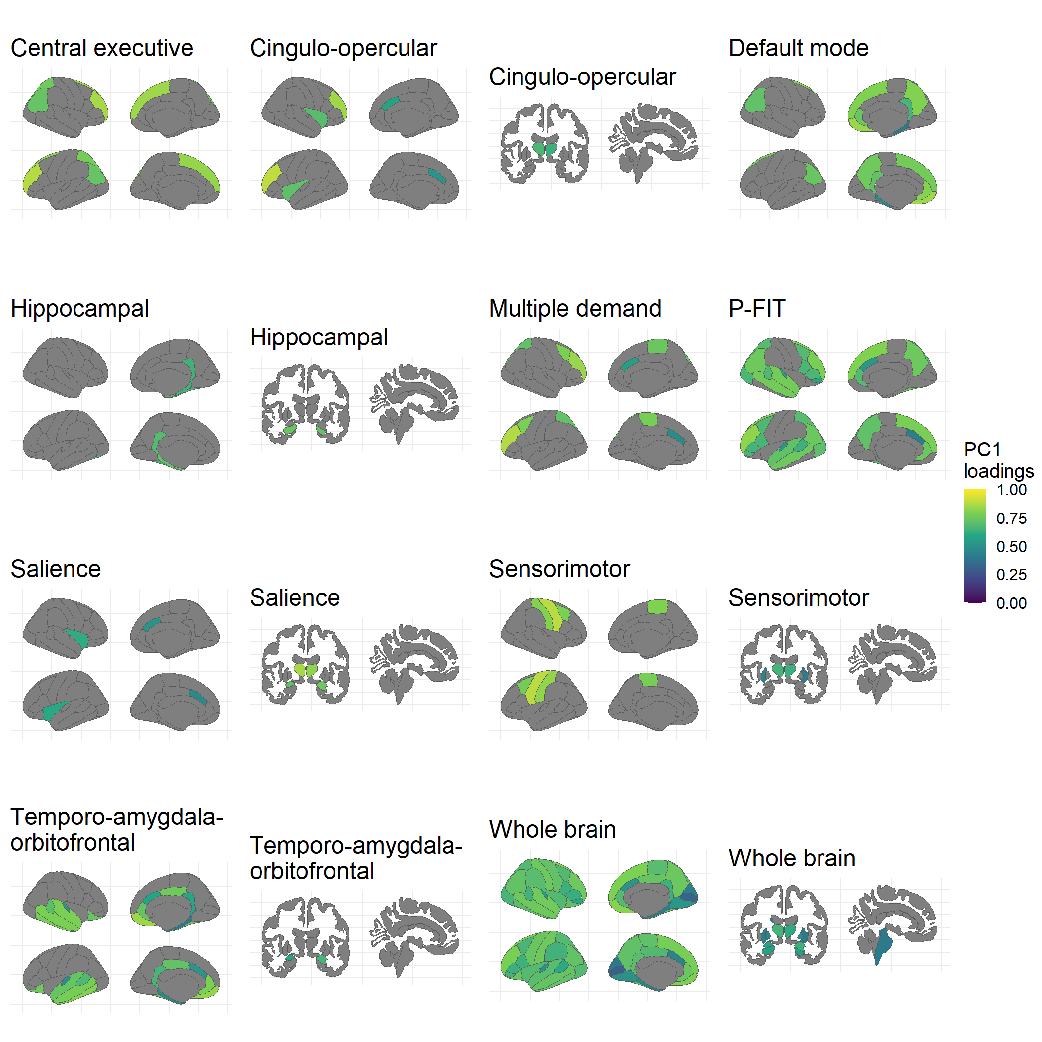
# tiff("C:/Users/k1894405/OneDrive - King's College London/PhD/Projects/Genomic SEM project/Revisions HBM/images/PC1loadings.tiff", width = 11, height = 11, units = 'in', res=1000)
# ggarrange(plotlist = plots, common.legend = TRUE, legend = "right")
# dev.off()![]()
By Anna Elisabeth Fürtjes
anna.furtjes@kcl.ac.uk